A densely connected LDCT image denoising network based on dual-edge extraction and multi-scale attention under compound loss

Abstract

BACKGROUND:

Low dose computed tomography (LDCT) uses lower radiation dose, but the reconstructed images contain higher noise that can have negative impact in disease diagnosis. Although deep learning with the edge extraction operators reserves edge information well, only applying the edge extraction operators to input LDCT images does not yield overall satisfactory results.

OBJECTIVE:

To improve LDCT images quality, this study proposes and tests a dual edge extraction multi-scale attention mechanism convolution neural network (DEMACNN) based on a compound loss.

METHODS:

The network uses edge extraction operators to extract edge information from both the input images and the feature maps in the network, improving the utilization of the edge operators and retaining the images edge information. The feature enhancement block is constructed by fusing the attention mechanism and multi-scale module, enhancing effective information, while suppressing useless information. The residual learning method is used to learn the network, improving the performance of the network, and solving the problem of gradient disappearance. Except for the network structure, a compound loss function, which consists of the MSE loss, the proposed joint total variation loss, and the edge loss, is proposed to enhance the denoising ability of the network and reserve the edge of images.

RESULTS:

Compared with other advanced methods (REDCNN, CT-former and EDCNN), the proposed new network achieves the best PSNR and SSIM values in LDCT images of the abdomen, which are 33.3486 and 0.9104, respectively. In addition, the new network also performs well on head and chest image data.

CONCLUSION:

The experimental results demonstrate that the proposed new network structure and denoising algorithm not only effectively removes the noise in LDCT images, but also protects the edges and details of the images well.

Keywords

Low dose CT(LDCT)image denoising edge operator attention mechanism residual learning convolution neural network (CNN)

1 Introduction

Computed Tomography (CT) plays a very important role in modern medical diagnosis. However, the radiation hazards from the X-ray have attracted more and more people’s attention [1, 2]. The high dose radiation generated during CT scanning cause harm to the human body. Seriously, it even causes various cancers. Low dose CT (LDCT) technology is an effective method to reduce the radiation hazard to human body. As the radiation dose decreases, the quality of the reconstructed images decreases, with many artifacts and noise. Degraded images are not sufficient for clinical diagnosis [3 –6].

In recent years, Convolutional neural network (CNN) has been verified to have good potential to solve the images denoising task and obtains better performance than most of the current traditional methods [7, 8]. Chen, et al. have proposed a fully connected CNN which maps LDCT images to corresponding normal dose CT (NDCT) images [9]. The denoising method has exceeded the traditional methods substantially, but the network has a problem of gradient disappearance. They have proposed an encoder-decoder convolutional network with residual connection (RED-CNN) [10]. By using the deconvolution network and fast connection, RED-CNN has solved the problem of gradient disappearance. Although RED-CNN has achieved good objective values, the denoised images are over-smoothed. Yang, et al. have proposed a generation adversarial network with Wasserstein distance and perception loss, which improves the phenomenon of images over-smooth [11]. Li, et al. have proposed an unpaired convolutional neural network for denoising low-dose CT images [12]. Park, et al. have used the improved U-net network to achieve end-to-end mapping between low- and high-resolution images [13]. Zhang, et al. have proposed a network based on dense connection and deconvolution (DD-Net), which uses fast connection to speed up the training speed of the network and improves the expressive ability of the network [14]. You, et al. have proposed a generation adversarial network based on cycle-consistency (GAN-Cycle), which strengthens the consistency between the output images and input images and finally recovers the high-resolution images from the LDCT images efficiently [15]. Wang, et al. have proposed a non-convolution visual transformer (CT-former) for LDCT images denoising which preserves the local context information well [16]. Liu, et al. have proposed a diffusion probabilistic prior for Low-Dose CT images Denoising, which is based on denoising diffusion probabilistic model - a powerful generative model [17], but the model does not perform well in preserving the edge information of the images.

In many previous research studies, edge information and attention mechanism have been verified to be useful to improve the performance of images processing tasks. Wang, et al. have proposed a ship images classification method by using edge extraction operators and multi-scale modules [18], improving classification accuracy. Woo, et al. have proposed a Convolutional Block Attention Module (CBAM) to improve the classification accuracy by using channel attention and spatial attention mechanisms [19]. Liang, et al. have proposed a dense connection network based on edge enhancement and a compound loss for low-dose CT denoising [20], which better preserves the edge information in the process of noise reduction. Luthra, et al. have proposed a visual transformer denoising network based on edge enhancement (E-former) [21], to enhance the edge information of the restored images to obtain higher quality images. However, these algorithms only perform edge extraction on the input images, ignoring the role of the feature map in the network training.

Inspired by the good performance of the edge operators in edge preservation and the success of multi-scale attention mechanisms in classification tasks, this paper proposes a dual edge extraction densely connected CNN network based on multi-scale attention mechanism for LDCT images denoising.

2 Materials and methods

2.1 Dataset and LDCT image noise description

In the experimental study, a dataset from the 2016 NIH AAPM-Mayo Clinic LDCT Challenge is used. It contains paired normal-dose CT (NDCT) images from 10 patients and synthesized one-quarter dose abdominal CT images, one-quarter dose head CT images, and one-tenth dose of chest images.

LDCT images denoising is seen as a mapping problem from LDCT images to NDCT images. Assuming z ∈ R^m×n represents a LDCT image and x ∈ R^m×n represents the corresponding NDCT image, z is expressed as:

$z = σ (x)$ (1) where σ is a complex degradation process. In addition, the denoising problem is transformed to find an optimal approximation function of σ^-1. It is expressed as f, which is expressed as: $\underset{f}{arg min} {∥ f (z) - x ∥}_{2}^{2}$ (2) where f stands for the network model and refers to the end-to-end mapping function. Deep learning removes noise by the training network. So, the mapping function f is estimated by the method based on deep learning.

The contributions of this paper are summarized as follows: The learnable edge convolutional operators with multiple directions are used to extract the edge from both the input images and the feature map obtained in the training process, which enable feature reuse and strengthen the edge information of the restored images.

The multi-scale module and attention module form a new module, named MA module. The MA module makes full use of the multi-scale information in images and focuses on important features. It reduces noise interference and improves the generalization ability of the model.

The residual noise learning method is used for training network, which improves the performance of the network and avoids the disappearance of gradient. The corresponding experiments have been implemented in this paper to prove that the residual learning method is superior to the traditional learning method for medical images denoising.

A new compound loss function which is composed of MSE loss, a total variation based joint loss and edge loss is introduced in the training stage. By using the proposed loss function, the denoising ability and edge preservation ability of the network are further improved.

2.2 Edge extraction module

Edge information is helpful to preserve details and edges in images denoising task [22]. Due to its good performance in edge detection, the learnable Sobel operators are used as edge extraction block in the proposed network. As shown in Fig. 1(a), the Sobel operators have four sub-templates with four directions including 0°, 90°, 45° and 135°. A learnable factor α is designed to control edge extraction intensity, which is more flexible and applicable compared with the traditional Sobel operators with fixed parameters.

Fig. 1

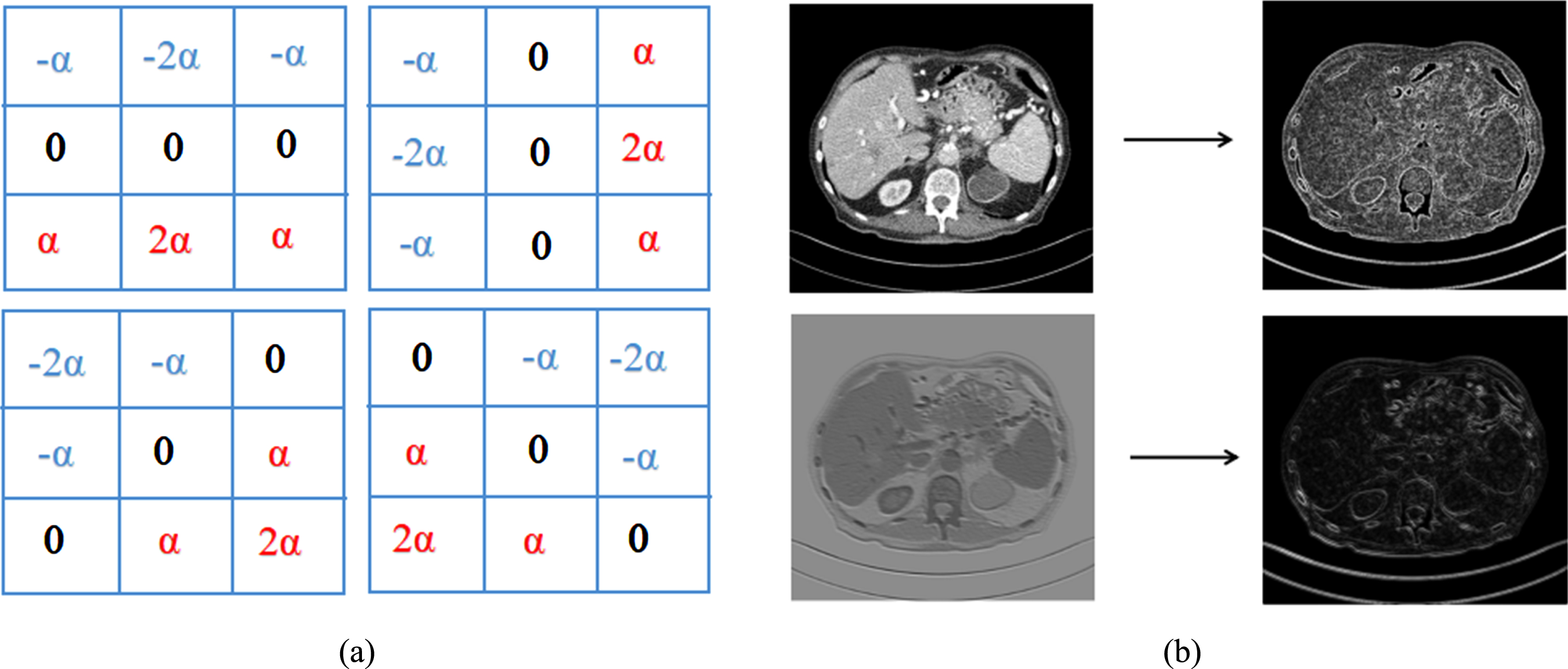
(a) Four different sets of Sobel operators (b) An example of edge extraction from the input image and the feature map, respectively.

Different from other methods, in this paper the edge information is extracted by using the learnable Sobel operators not only from the input images, but also from the feature maps obtained in the network. To better illustrate our point of view, the visualization results of edge extraction on the input images and the feature maps are shown in Fig. 1(b). The top one is the result after edge extraction of LDCT image and the bottom one is from the feature map obtained after four 3 × 3 convolutions. In Fig. 1(b) we see that after the edge extraction of the feature map, the edge information of the image is still available and contains less noise. In other words, the edge features obtained from the feature maps not only contain the edge information of the original images, but also can resist noise compared to the edge features of the original images. Therefore, the edge information is better utilized by fusing with the edges of the original images and the edges of feature maps. The edges of the denoised images are better preserved.

To verify our idea, the actual thoracic phantom is used for experiments. The results are shown in Fig. 2 as shown below. In the left column, from top to bottom, the images are NDCT images, LDCT images and the feature maps extracted from the low-dose images (the output of the fourth convolutional layer), respectively. The images in the right column are the corresponding edge images extracted from the left column. From Fig. 2, in the LDCT images, there are lots of artifacts and noise compared to the NDCT images. In addition, we see that the edge images extracted from the LDCT images are severely disturbed by noise, whereas the edge images extracted from the feature maps not only contain the edge information like the one of NDCT images, but also contain less noise than the edge information of LDCT images.

Fig. 2

Results of edge extraction on the modal image.

2.3 Multi-scale attention module (MA module)

The MA module is composed of multi-scale module and attention module. By combing the advantages of spatial attention, channel attention and multi-scale features, the MA module increases the ability of the network to extract features and enables the network to focus on the important information of the images.

2.3.1 Multi-scale module

In general, the performance of CNN is improved by increasing the convolution layers. However, the network parameters increase greatly, and the gradient disappearance phenomenon is prone to occur [23, 24]. In addition, when the training data set is small, the trained network is likely to over-fit. Muti-scale network architecture alleviates the above-mentioned problems to a large extent [25]. Inspired by [26], the multi-scale module designed in this paper is shown in Fig. 3.

Fig. 3

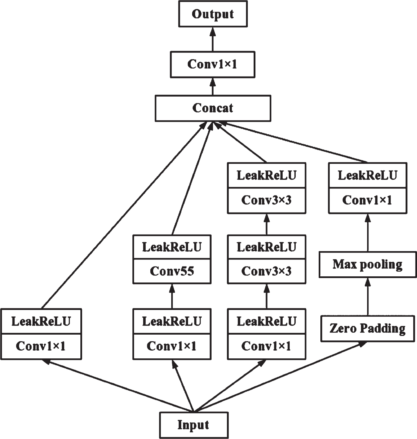
Multi-scale module designed in this paper.

Each convolution layer is activated by the LeakReLU layer to maintain non-linearity. For the rightmost branch, a zero-padding operation is performed on the input images before pooling to ensure that the pooled result matches the output size of the other three convolutional layers. The convolution kernel of different sizes is combined to improve the feature extraction ability of the network. In addition, each path uses a 1 × 1 convolution kernel for reducing the number of parameters and avoiding the problem of excessive computation.

2.3.2 Attention module

In general, the attention mechanism of deep learning selects a small amount of important information from many available data and focuses on important details. It suppresses unimportant information to improve network performance. CBAM is a simple and effective attention module. Given an intermediate feature map, the CBAM module infers the attention map sequentially along two independent dimensions (channel and space) and multiplies the attention map with the input feature map for feature optimization. Referring to [19], the attention model shown in Figs. 4 5 is adopted.

Fig. 4

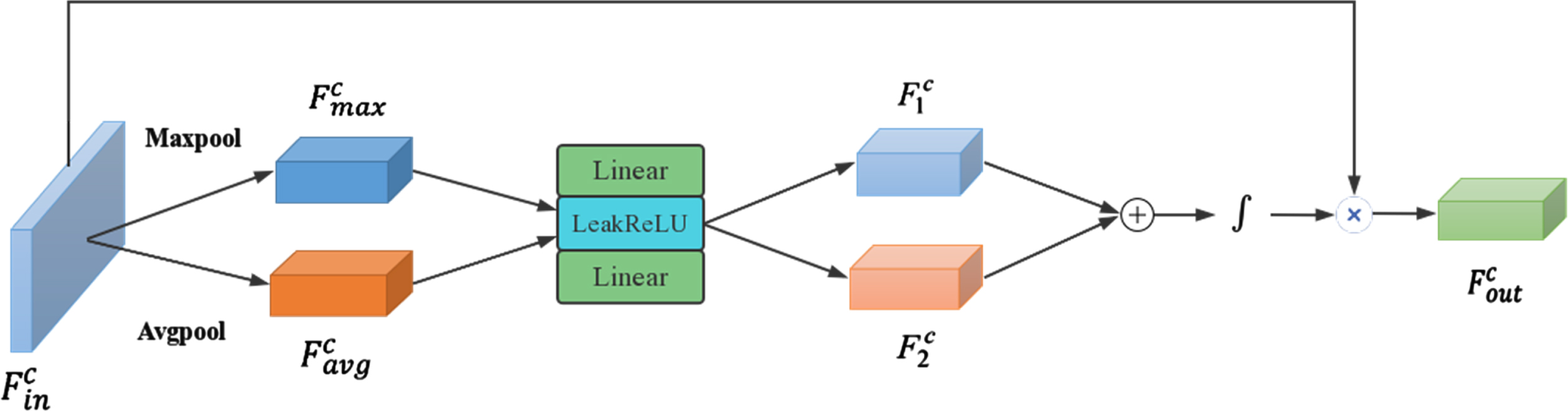
Channel attention network structure.

Fig. 5

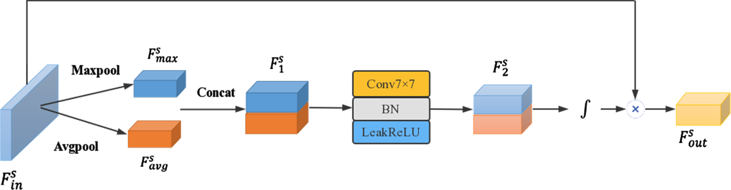
Spatial attention network structure.

The main purpose of the channel attention module is to pay more attention to the effective feature channel of the network. Through the average pooling layer and the maximum pooling layer, the input features $F_{in}^{c} \in R^{H \times W \times C}$ generate the average pooling feature $F_{avg}^{c} \in R^{1 \times 1 \times C}$ and the maximum pooling feature $F_{max}^{c} \in R^{1 \times 1 \times C}$ . Then the two features are entered into the shared multi-layer perceptive network to get $F_{1}^{c} \in R^{1 \times 1 \times C}$ and $F_{2}^{c} \in R^{1 \times 1 \times C}$ , which are respectively expressed as follows. $F_{1}^{c} = W_{2} (φ (W_{1} (F_{avg}^{c})))$ (3) $F_{2}^{c} = W_{2} (φ (W_{1} (F_{max}^{c})))$ (4) where W₁ and W₂ are the weight values, φ represents the LeakReLU activation function. The output of the channel attention module is expressed as: $F_{out}^{c} = F_{c}^{in} \otimes sig (F_{1}^{c} \oplus F_{2}^{c})$ (5) where ⊕ represents a pixel-by-pixel summation operation and ⊗ represents a pixel-by-pixel multiplication operation. sig represents the Sigmoid activation function which non-linearly normalizes the attention map to [0,1]. By using the element summation operation, $F_{1}^{c}$ and $F_{2}^{c}$ are merged. After the Sigmoid operation, the channel attention feature $F_{out}^{c} \in R^{H \times W \times C}$ is obtained by multiply the original input feature $F_{in}^{c}$ pixel-by-pixel. The symbol ∫ represents Sigmoid operation in Figs. 4 5.

The spatial attention module uses the spatial relationship between features to focus on the information of features. Therefore, the spatial attention module is a supplement to the channel attention module. The input feature $F_{in}^{s} \in R^{H \times W \times C}$ is entered into the global average pooling layer and global max pooling layer to generate two new features $F_{avg}^{s} \in R^{H \times W \times 1}$ and $F_{max}^{s} \in R^{H \times W \times 1}$ . Then, $F_{avg}^{s}$ and $F_{max}^{s}$ are spliced to get a feature $F_{1}^{s} \in R^{H \times W \times 2}$ . Followed, use 7 × 7 convolution kernel, BN layer and LeakReLU layer successively to generate feature $F_{2}^{s} \in R^{H \times W \times 2}$ . The BN operator increases the gradient and makes the network converge fast. The output of the spatial attention model is expressed as:

$F_{out}^{s} = F_{in}^{s} \otimes sig (F_{2}^{s})$ (6)

According to formula 6, the spatial attention feature $F_{out}^{s} \in R^{H \times W \times C}$ is obtained.

2.4 Residual learning

Deep neural networks lead to gradient problems, training difficulties, degradation of network performance, and waste of resources [27 –29]. Residual learning solves the problem of deep network degradation and improves the convergence speed of the network [30, 31]. The goal of residual learning is to implicitly remove latent clean images in the hidden layer. Input a noise image x = y + v into our network, here x is the noise image. In our paper, it is an LDCT image. y is true value and is residual noise. Our network does not directly output the denoised image $\hat{y}$ but predicts the residual v image $\hat{v}$ which is the difference between the LDCT image and the NDCT image. According to literature [32], when the original mapping is close to the identity mapping, the residual mapping is easier to optimize. Different from the general denoising model which aims at learning the mapping function of $F (x) = \hat{y}$ , in the proposed method we use the residual formula to train our network learning residual mapping $R (x) = \hat{v}$ . Finally, the denoised image is obtained through $\hat{y} = x - R (x)$ . Content-Noise Complementary Learning (CNCL) employs a specific architecture that uses separate networks for content and noise so that they learn complementary information [33].

In contrast, residual noise learning typically uses residual connections in a single network to learn residual noise representations. Residual noise learning focuses on learning residual noise representations to improve denoising performance effectively. To verify the effectiveness of residual learning in medical images denoising, the paper also compares it with deterministic learning, which is described in the experiments part.

2.5 The proposed network architecture

Overall, a dual edge extraction densely connected CNN network based multi-scale attention model (DEMACNN) is proposed for LDCT images denoising. The architecture of the proposed network is shown in Fig. 6.

Fig. 6

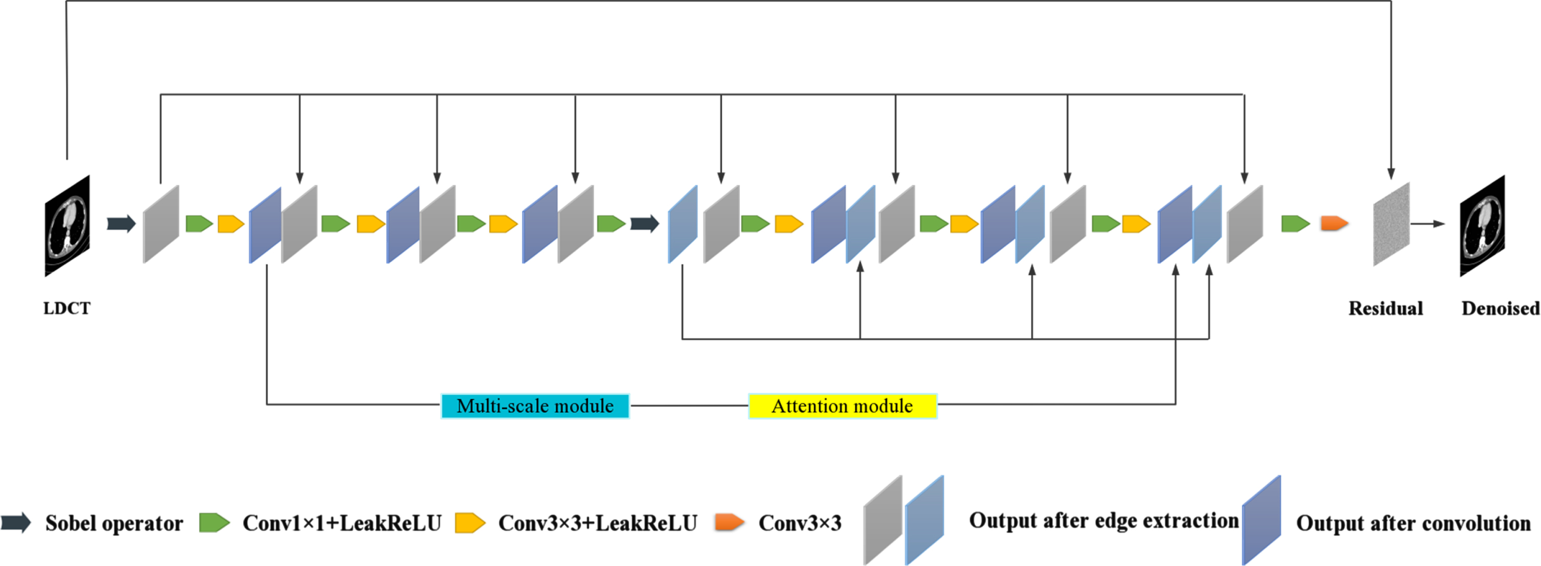
Proposed overall network architecture.

The trainable Sobel operators are used for both the input images and the feature maps. The number of trainable Sobel operators is 32. In the network, dense connections are used to make full use of the extracted edge information and original input [34]. Specifically, as shown in Fig. 6, we convey the output of the Sobel operators to each convolution block through skip connection and concatenate them in the channel dimension. Except for the last layer, the convolutional layer consists of convolutional kernels of size 1 × 1 and 3 × 3, and the number of convolutional filters is all set to 32.

In the last layer, the number of 3 × 3 convolutional filter is 1 for obtaining the output of a single channel. The activation function is LeakReLU. In each block, the output of the previous layer and the output of Sobel operators are fused using convolution with a 1 × 1 kernel, and features in the images are typically learned using convolution with a 3 × 3 kernel. The MA module, which integrates a multi-scale module and an attention module, is to increase the depth of the network and obtain more effective information. We import the result of the first 3 × 3 convolutional layer into the MA module and fuse the output of MA module with the result of the sixth 3 × 3 convolutional layer. In addition, to keep the output size the same as the input size, we pad the feature mapping in the model to ensure that the space size does not change during forward propagation. The predictable result of the network is the residual noise and the final denoising image is obtained by connecting the residuals.

2.6 Loss function

Mean-square error (MSE) is a loss function, and it is widely used in various deep learning methods, which calculates the average of the squared differences between the predicted and true values. It is expressed as: $L_{mse} = \frac{1}{N} \sum_{i}^{N} {∥ F (x_{i}, θ) - y_{i} ∥}^{2}$ (7) where x_i are the i-th pixel of input images x, y_i are the pixel of the target images y, N is the total number of pixels in x_i, F (x_i, θ) are the denoised result of x_i with parameter θ in the network.

Although wildly used in images restoration tasks, MSE loss has some disadvantages. For example, the evaluation index of MSE has no good correlation with the subjective perception of the images. Because it considers the average values and does not consider the influence of some significant features.

This paper introduced a joint total variation loss function which is better representation the sparsity of images and an edge loss function which well considers high-frequency texture structure information and improves images detail performance.

The joint total variation loss is constructed based on the total variation loss (TV Loss), which shows the advanced performance in improving images sparsity and reducing noise in the image’s restoration task [35, 36]. The proposed joint constraint loss L_JTV is defined as: $L_{JTV} = τ {∥ F (x_{i}, θ) ∥}_{TV} + (1 - τ) {∥ y - F (x_{i}, θ) ∥}_{TV}$ (8) where τ is a weighting parameter. The above constraint combines two parts: the first part is used to sparse the reconstructed image and reduce obvious artifacts. The second part is used to minimize the difference image to reserve image features [37].

To determine the weighting parameter factor τ in the joint total variation loss function, we select the parameter τ from {0, 0.1, 0.3, 0.5, 1.0}. The results of the experiment are shown in Fig. 7. The results show that the weighting parameter τ= 0.5 achieves the lowest loss, which is used in following experiments, and the two components of the joint total variation loss the two components of the joint total variation loss need to be jointly minimized under a bidirectional constraint.

Fig. 7

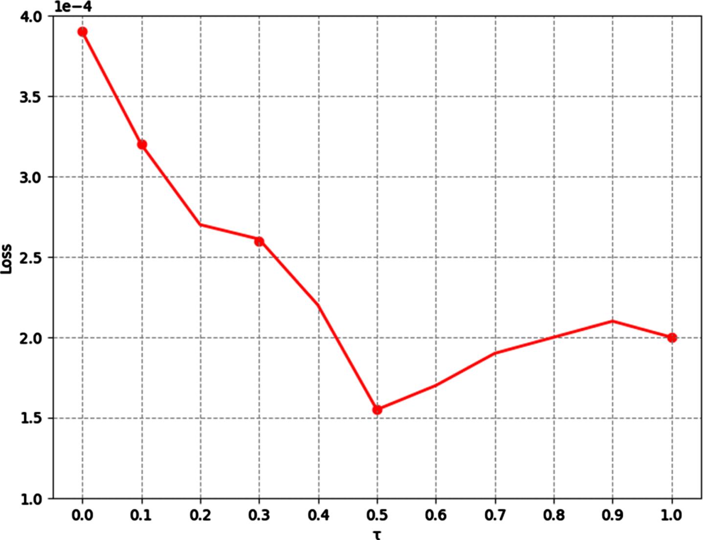
The effect of parameter τ on training loss.

The edge loss function is expressed as follows: $L_{edgeloss} = \frac{\sum_{i = 1}^{W} \sum_{j = 1}^{H} E_{i, j} \cdot | F (x_{i, j}, θ) - y |}{WH}$ (9) where F (x_i,j, θ) and y are network output images and target images respectively, E_i,j is the edge feature obtained from target images, W and H represent the width and height of the image, respectively. The subscripts i and j are the row and column coordinates of the pixel x, respectively. The E_i,j is extracted by the Sobel operators. In formula (9), the edge loss is calculated by multiply E_i,j and the difference between F (x_i,j, θ) and y. Specifically speaking, to form the edge loss component, we first apply the Sobel operators to the target image y to obtain the edge mapping E_i,j. The edge loss is then calculated as the average of the product of the edge mapping E_i,j and the reconstruction error [38]. Through this operation, the edge information of restored image is enhanced by the loss function.

Finally, our network is fine-tuned end-to-end to minimize the following objective functions: $L_{total} = L_{mse} + β_{1} L_{JTV} + β_{2} L_{edgeloss}$ (10) where β₁ and β₂ are the parameters to balance different loss functions.

Similarly, we select the parameter β₁, β₂ from {0, 0.05, 0.1 0.2, 0.3, 0.4, 0.5}. The results of the experiment are shown in Fig. 8, which shows that for the joint total variation loss, the lowest loss is obtained when β₁= 0.1, while for the edge loss, the lowest loss is obtained when β₂= 0.05, which is used in following experiments.

Fig. 8

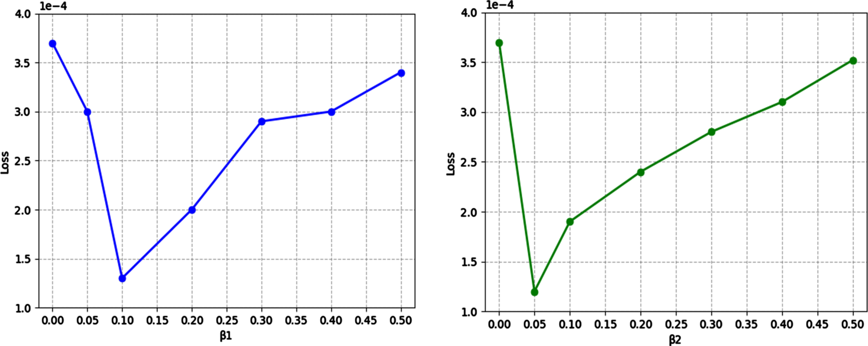
The effect of parameter β₁, β₂ on training loss.

3 Experiment and results

3.1 Experimental data

The number of slices in the data set is 2080. The size of image is 512 × 512. The network uses the supervised training process. In terms of data preparation, this paper uses a k-fold cross-validation approach to train and test the network. First, the data from 10 patients are randomly disrupted to avoid the effect of data order on cross-validation. Then, the data set is divided into k = 5 copies. For each k, select the k-th copy as the test set and the remaining k-1 copies as the training set. Therefore, the number of training sets in this paper is 1664 and the number of test sets is 416. This paper uses the training set to train the model and uses the test set to evaluate the performance of the model. Repeat until each k has been used as a test set. The mean value of k cross-validation results is calculated as the result of all model performance evaluation.

3.2 Experimental setup

This paper is based on the implementation of the Pytorch framework. The convolution layer in this model uses the default random initialization and the Sobel operators of all edge extraction modules are initialized to 1 before training. Conclusion based on section 3.5, the τ in the loss function L_JTV is set to 0.5. The joint variation coefficient β₁ in the overall loss function defined in formula (10) is 0.1 and the edge loss coefficient β₂ is 0.05. In the optimization process, the default configuration of the Adam optimizer is used. Batch size is 16 and the Epoch is 200. In this paper, the initial learning rate is set to 0.0001, and a learning rate decay factor γ= 0.5 is defined, which means that during the training process, the learning rate decreases to half of the original one after every 3000 iterations. When testing the model, use the 64 × 64 LDCT images as the input and directly output the denoising results. The running environment is Pytorch 1.11, Windows 10, CUDA11.3, NVIDA GeForce RTX 3080GPU.

3.3 Experimental results

This section shows the experimental results. Three related algorithms including REDCNN, CT-former and EDCNN are used for comparison. In this paper, the objective indicators of the four models are calculated by using Peak Signal to Noise Ratio (PSNR), Structural Similarity (SSIM) and Root Mean Square Error (RMSE). The unit of PSNR is dB. A higher PSNR value means better image denoising effect. Higher SSIM value means higher similarity between the denoised image and the NDCT image. RMSE value represents the error between the denoised image and the NDCT image. The smaller the RMSE value, the better the quality of the recovered image.

Objective comparison results of these methods are shown in Table 1 3(including the abdomen, head, and chest datasets). In this paper, objective indicators are calculated as the average of five cross-validation results. Figure 9 shows the results of our five cross-validation, from which it is seen that the results of the five tests are similar. The difference between the highest PSNR value and the lowest PSNR value is about 0.26, the difference between the highest SSIM value and the lowest SSIM value is about 0.0033, and the difference between the highest RMSE value and the lowest RMSE value is about 0.3. The LDCT represents the original input image, which contains lots of artifacts and noise. In Tables 2 6, LDCT represents the same meaning. It is seen that the proposed DEMACNN model obtains the two highest values compared with other related models in Table 1. The proposed DEMACNN models obtain the highest average SSIM value and the second highest average PSNR value compared to other related models in Tables 2 3. In addition, when adding the residual learning to the DEMACNN, the performance of the proposed network is further improved, and the objective values are improved. It indicates that the proposed DEMACNN algorithm shows more proficiency in LDCT image denoising.

Table 1
Comparison of the mean value of objective indicators of different models in after five cross-validations(abdomen)

Methods AVGPSNR AVGSSIM AVGRMSE

LDCT 29.7432 0.8632 13.2648

REDCNN 32.9613 0.9060 9.1279

EDCNN 32.8770 0.9071 9.3651

CT-former 32.8997 0.9054 9.2185

DEMACNN 33.1516 0.9081 8.9188

DEMACNN+residual 33.3486 0.9104 8.7736

Methods	AVGPSNR	AVGSSIM	AVGRMSE
LDCT	29.7432	0.8632	13.2648
REDCNN	32.9613	0.9060	9.1279
EDCNN	32.8770	0.9071	9.3651
CT-former	32.8997	0.9054	9.2185
DEMACNN	33.1516	0.9081	8.9188
DEMACNN+residual	33.3486	0.9104	8.7736

Table 2

Comparison of the mean value of objective indicators of different models after five cross-validations(head)

Methods	AVGPSNR	AVGSSIM	AVGRMSE
LDCT	38.6625	0.9473	2.6319
REDCNN	40.2078	0.9620	2.1349
EDCNN	39.9513	0.9623	2.4080
CT-former	38.8432	0.9583	2.5124
DEMACNN	39.9968	0.9645	2.1646
DEMACNN+residual	40.1952	0.9680	2.1410

Table 3

Comparison of the mean value of objective indicators of different models after five cross-validations(chest)

Methods	AVGPSNR	AVGSSIM	AVGRMSE
LDCT	20.4182	0.8235	67.7013
REDCNN	27.8463	0.8426	28.5100
EDCNN	27.0360	0.8538	31.2679
CT-former	25.9417	0.8374	33.7165
DEMACNN	27.6215	0.8569	29.2433
DEMACNN+residual	27.8236	0.8614	28.8053

Fig. 9

Results of the cross-validation test for DEMACNN+residual.

Table 4

Performance comparison on model structure

Methods	AVGPSNR	AVGSSIM	AVGRMSE
LDCT	29.7432	0.8632	13.2648
BCNN	32.4952	0.8926	9.8459
BCNN+TEI	32.6226	0.9009	9.3857
BCNN+TEI+TEF	32.7513	0.9028	9.3168
BCNN+EI	32.8297	0.9057	9.2792
BCNN+EI+EF	32.9883	0.9075	9.1445
BCNN+EI+EF+MA	33.1103	0.9080	9.1000

Table 5

Model Structure Performance Comparison in RENDCNN

Methods	AVGPSNR	AVGSSIM	AVGRMSE
LDCT	29.7432	0.8632	13.2648
REDCNN	32.9705	0.9066	9.1204
REDCNN+EI	33.0699	0.9073	9.0011
REDCNN+EI+EF	33.1014	0.9075	9.0007
REDCNN+EI+EF+MA	33.1217	0.9081	8.9742

Table 6

Research on the number of MA blocks

Methods	AVGPSNR	AVGSSIM	AVGRMSE
LDCT	29.7432	0.8632	13.2648
BCNN	32.8134	0.9053	9.2781
BCNN+MA	32.9426	0.9062	9.1448
BCNN+2MA	32.4313	0.8971	9.6135
BCNN+3MA	31.9572	0.8958	10.2321

The denoising abdominal, head and chest results of various algorithms are shown in Figs. 10 12. In order to observe the details of the image more clearly, the region of interest which is marked in the red box in Figs. 10(a1)-(f1) 12(a1)-(f1) is enlarged. We also label the objective indicators for the denoising results of each method in Figs. 10 12.

Fig. 10

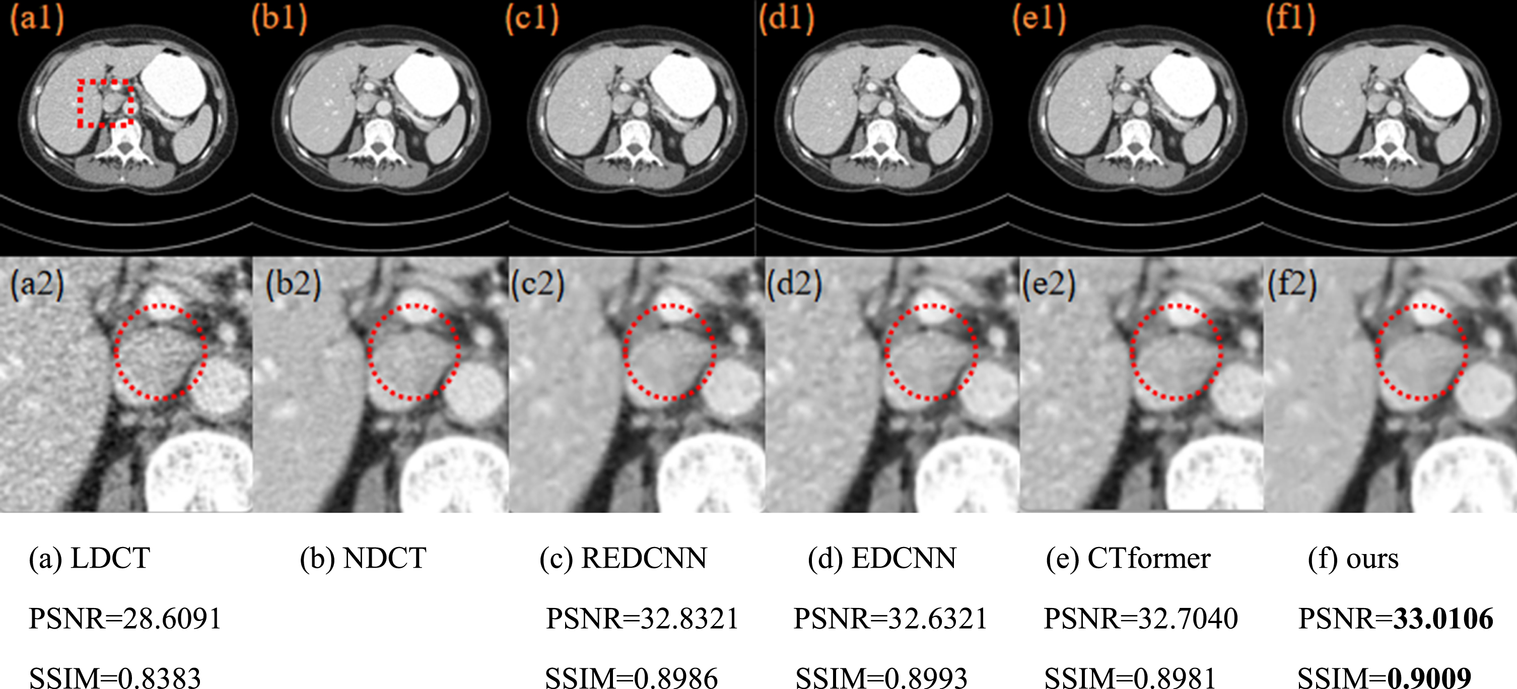
The denoising results of different models in abdomen images and the region of interest (ROI) in the red box is enlarged.

Fig. 11

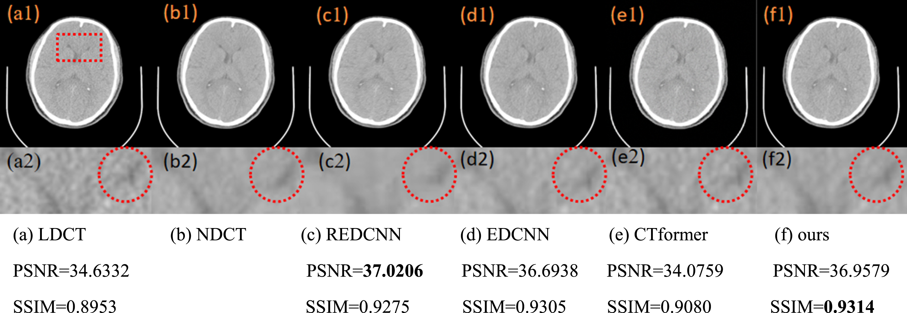
The denoising results of different models in head images and the region of interest (ROI) in the red box is enlarged.

Fig. 12

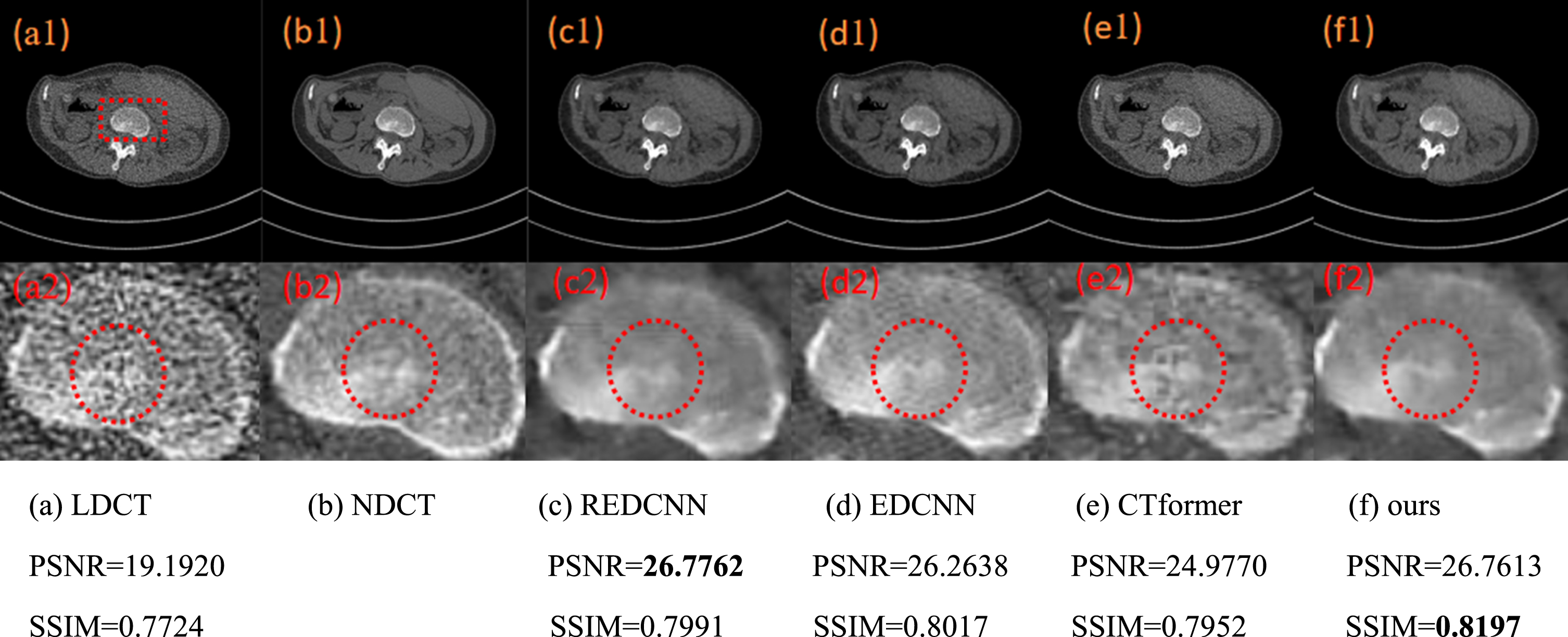
The denoising results of different models in chest images and the region of interest (ROI) in the red box is enlarged.

Figure 10(a) is the abdomen LDCT image and Fig. 10(b) is the corresponding NDCT image. Figure 10(c1)-(f1) are the denoising results of REDCNN, EDCNN, CT-former and the proposed method respectively. It is seen that there are more noises in Fig. 10(a2) than Fig. 10(b2). It is seen from Fig. 10(c1) and 10(c2) that REDCNN removes the noise well, but the edges and details of the image are blurred. The edge information of Fig. 10(d2) and 10(e2) are well preserved but there are still residual noises. In Fig. 10(f2), we see that the proposed algorithm strikes a better balance between noise removal and edge preservation. In the region marked by the red circle the edge of our method is much closer to the NDCT image. The edge of other methods is much closer to the one of LDCT image, in which the image edge is disturbed by noise. It is also seen from the objective indicators that the proposed method achieves a PSNR value of 33.0106 and a SSIM value of 0.9009, both of which are better than the compared methods.

Figure 11(a) shows the head LDCT image and Fig. 11(b) shows the corresponding NDCT image. Figure 11(c1)-(f1) show the denoising results of REDCNN, EDCNN, CT-former and the proposed method in this paper, respectively. It is seen that there are more noises in Fig. 11(a2) than in Fig. 11(b2). From Fig. 11(c1) and 11(c2), it is seen that REDCNN removes the noise well, but the edges and details of the image are over-smoothing. Figure 11(d2) has better preservation of edge information, but there is still residual noise. In Fig. 11(e2), there are more noises into the image in CTformer, making it difficult to distinguish the density distribution of this tissue. In Fig. 11(f2), we see that the proposed algorithm strikes a better balance between noise removal and edge preservation. In the region marked by the red circle the edge and detail of our method is much closer to the NDCT image. It is also seen from the objective indicators that the proposed method achieves the second best PSNR value of 36.9579 and the best SSIM value of 0.9314.

Figure 12(a) shows the chest LDCT image and Fig. 12(b) shows the corresponding NDCT image. Figure 12(c1)-(f1) show the denoising results of REDCNN, EDCNN, CT-former and the proposed method in this paper, respectively. It is seen that there are more noises in Fig. 12(a2) than 12(b2). From Fig. 12(c1) and 12(c2), it is seen that REDCNN is better, however, there is obvious over-smoothing phenomenon at the edges. CTformer has obvious residual noise. EDCNN and the proposed DEMACNN are effective in recovering the details and overall structure, and DEMACNN performs better than EDCNN in suppressing artifacts. It is also seen from the objective indicators that the proposed method achieves the second best PSNR value of 26.7613 and the best SSIM value of 0.8197.

3.4 Ablation study

In this section, we compare and analyze the performance of our model under different structures and loss function configurations.

3.4.1 Network structure

To explore the influence of each part in the DEMACNN model, a decomposition experiment on its structure is carried out in this section. For the convenience of description, we define six networks’ abbreviations bellow.

BCNN: A basic network which removes the MA module and the two edge extraction modules from the structure shown in Fig. 6 and uses MSE loss to guide network training.

TEI: TEI module refers to the edge extraction of the input images using the traditional Sobel operators with fixed parameters.

TEF: TEF module refers to the edge extraction of the feature maps by using the traditional Sobel operators with fixed parameters.

EI: The EI module refers to using the learnable Sobel edge operators to extract the edge of the images.

EF: The EF module refers to using the learnable Sobel edge operators to extract the edge of the feature maps.

BCNN+TEI: A network by adding the TEI module to BCNN.

BCNN+TEI+TEF: A network by adding the TEI and TEF module to BCNN.

BCNN+EI: A network by adding the EI module to BCNN.

BCNN+EI+EF: A network by adding the EI module and EF module to BCNN.

BCNN+EI+EF+MA: The proposed network DEMACNN, which is constructed by adding EI module, EF module and MA module to BCNN.

Table 4 shows the PSNR, SSIM and RMSE values of the six networks mentioned above. From Table 4, it is seen that as TEI, TEF, EI, EF and MA modules are added sequentially to the base network BCNN, the objective indicators values increase sequentially and BCNN+EI+EF+MA (DEMACNN) obtains the highest PSNR, SSIM values and it has the lowest RMSE values. Table 4 also shows that the learnable Sobel edge operators achieve better results than traditional Sobel operators. This demonstrates that the learnable edge operators used in this paper perform better than the traditional edge operators.

Figure 13 shows the curves of PSNR values changing with the number of iteration epoch under BCNN, BCNN+EI, BCNN+EI+EF, BCNN+EI+EF+MA(DEMACNN) structures. It is worth noting that the PSNR values increase continuously by adding the EI module, EF module and MA module. In addition, the EI module, EF module and MA module accelerate the convergence process of the model.

Fig. 13

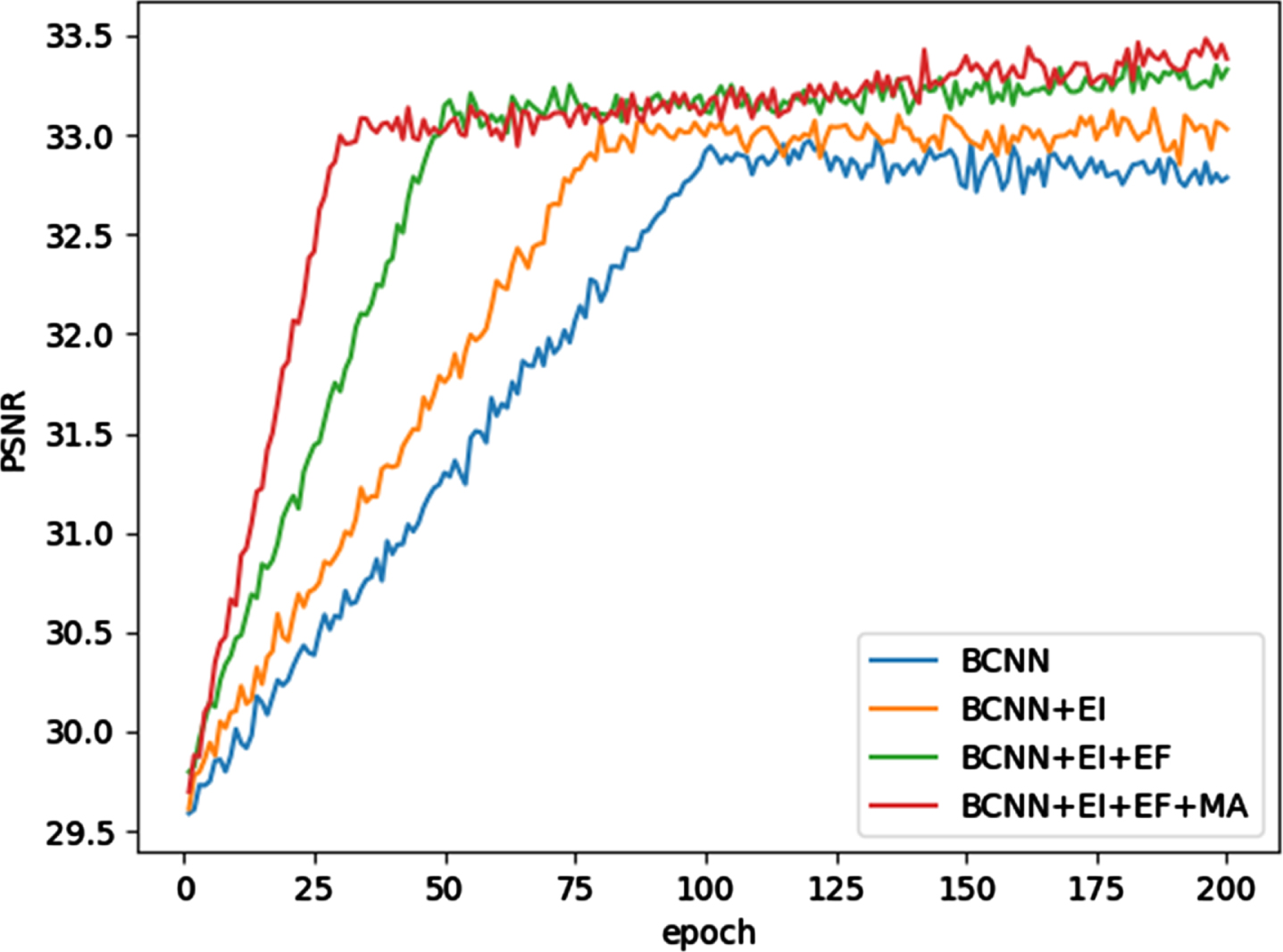
The PSNR curves in the training process.

The classic REDCNN network is used to further verify the effectiveness and generalization of the various modules in our network. We perform the EI, EF, and MA module on the REDCNN network, and the results are shown in Table 5 below, which shows that after adding the EI module, EF module and MA module sequentially to the REDCNN network, the values of the objective indicators obtained also increase sequentially, which proves the effectiveness and generalization of the three modules.

In addition, this paper explores the impact of the number of MA modules on the network. Based on the BCNN model, this paper adds MA modules between the output of the first 3 × 3 convolution kernel and the output of the sixth 3 × 3 convolution kernel (BCNN+MA). Based on BCNN+MA, adds a MA module between the output of the second 3 × 3 convolution kernel and the output of the fifth 3 × 3 convolution kernel (BCNN+2MA). Then, based on (BCNN+2MA), adds a MA module between the output of the third 3 × 3 convolution kernel and the output of the fourth 3 × 3 convolution kernel (BCNN+3MA). The results are shown in Table 6.

The objective denoising results of different networks including BCNN, BCNN+MA, BCNN+2MA and BCNN+3MA are shown in Table 6. It is seen that with the increase of MA modules, the performance of the network is declining. It is best to add only one MA block between the outputs of the first and the sixth convolution kernel. Moreover, adding one MA module to the BCNN network has fewer parameters than adding multiple MA modules, making the proposed network easier to train. Therefore, this paper adds one MA module.

3.4.2 Loss function

To prove the effectiveness of our loss function, in this section the MSE loss, the edge loss (eloss) and the ResNet50 perception loss (Res50) are used for comparison. For the convenience of description, we define the following symbolic representations.

MSE: Use the MSE loss function to guide the proposed DEMACNN network.

MSE+Res50: Use the MSE loss function and the ResNet50 perception loss to guide the proposed DEMACNN network.

MSE+eloss: Use the MSE loss function and edge loss function to guide the proposed DEMACNN network.

MSE+TV+eloss: Use the MSE loss function, traditional total variation loss function and edge loss function to guide the proposed DEMACNN network.

MSE+JTV+eloss: Use the proposed loss function which is defined in formula (10) to guide the proposed DEMACNN network.

The denoising results of the proposed DEMACNN network by using the above five different loss functions are shown in Fig. 14. We see that the edge information of Fig. 14(b) is blurred. Figure 14(c) and 14(d) are better preservation of the edge information but there are residual noises. Figure 14(e) and 14(f) strike a better balance between the edge information preservation and denoising effect. In addition, the joint total variation loss used in this paper achieves better results than the traditional total variation loss in the denoising effect and suppressing artifacts.

Fig. 14

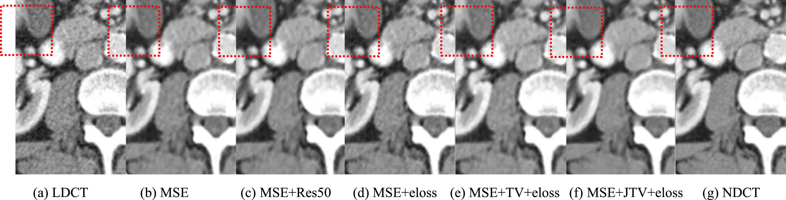
The visual effect of denoising with different loss functions (local area) and the area of interest (ROI) in the red box is selected to calculate objective indicators.

The objective indicators in the red box of Fig. 14 are shown in Table 7. It is seen that when adding the traditional total variation loss to the MSE+eloss function, MSE+TV+eloss obtains higher PSNR and SSIM values and lower RMSE value than MSE+eloss and MSE+Res50. In addition, when adding the joint total variation loss to the MSE+eloss function, MSE+JTV+eloss performs better objective indicators than MSE+TV+eloss. It proves the proposed joint total variation loss is effective.

Table 7

Comparison of different loss functions

Methods	PSNR	SSIM	RMSE
LDCT	29.2110	0.6166	0.0132
MSE	29.8939	0.7152	0.0119
MSE+Res50	30.0541	0.7824	0.0088
MSE+eloss	30.0746	0.7839	0.0074
MSE+TV+eloss	30.2581	0.8225	0.0062
MSE+JTV+eloss	30.7995	0.8479	0.0057

4 Conclusion

To sum up, this paper proposes an LDCT images denoising model based on multi-scale attention mechanism and the compound loss. In this paper, we use edge extraction module and multi-scale attention module to produce high quality images. Construct a joint total variation loss to enhance the denoising ability of the network and introduce an edge loss to preserve the edge information of the images. Use the residual learning method for training the network to avoid the disappearance of the gradient. The comparison with the previous models proves the effectiveness of our method.

Footnotes

Acknowledgments

This work was supported in part by (1) the State Council and the central government guide local funds of China under Grant YDZX20201400001547, (2) the Natural Science Foundation of Shanxi Province under Grant 202203021222015, and (3) Scientific and Technological Innovation Programs of Higher Education Institutions in Shanxi under Grant 2020L0051 and 2020L0048, and (4) Practice and Innovation Programs of Postgraduates in Shanxi Province under Grant 2023SJ011.

Ethics approval

Not applicable.

Conflicts of interest/Competing interests

We declare that we have no conflict of interest.

Availability of data and material

The data that support the findings of this study are available from TCIA (The Cancer Imaging Archive) but restrictions apply to the availability of these data, which were used under license for the current study, and so are not publicly available. Data are however available from the authors upon reasonable request and with permission of TCIA.

Code availability

The code can be made available on request.

Authors’ contributions

All authors developed the idea and accomplished the manuscript writing and performed the experiments. All authors read and approved the final manuscript.

References

Smith-Bindman

Radiation dose associated with common computed tomography examinations and the associated lifetime attributable risk of cancer, Arch Intern Med 169(22) (2009), 2078–2086. doi: 10.1001/archinternmed.2009.427

Yang

Y.Q.

and Fang

W.C.

Static superconducting gantry-based proton CT combined with X-ray CT as prior image for FLASH proton therapy, Nucl Sci Tech 34(1) (2023), 1–11. doi: 10.1007/s41365-022-01163-2

Brenner

and Hall

Computed tomography-an increasing source of radiation exposure, New Engl J Med 357 (2007), 2277–2284. doi: 10.1056/NEJMra072149

Donya

and Radford

Radiation in medicine: Origins, risks and aspirations, Global Cardiology Science and Practice 4(57) (2014), 437–448. doi: 10.5339/gcsp.2014.57

Eijnatten

M.V.

CT image segmentation methods for bone used in medical additive manufacturing, Medical Engineering Physics 51(1) (2017), 6–16. doi: 10.1016/j.medengphy.2017.10.008

Hobbs

J.B.

and Goldstein

Physician knowledge of radiation exposure and risk in medical imaging, Journal of the American College of Radiology 15(1) (2018), 34–43. doi: 10.1016/j.jacr.2017.08.034

Kan

E.J.

and Min

J.C.

A deep convolutional neural network using directional wavelets for low-dose X-ray CT reconstruction, Medical Physics 44(10) (2017), 360–375. doi: 10.1002/mp.12344

Zhang

and Zuo

W.M.

FFDNet: Toward a fast and flexible solution for CNN based image denoising, IEEE Transactions on Image Processing 27(9) (2018), 1–1. doi: 10.1109/TIP.2018.2839891

Chen

and Zhang

Low-dose CT via convolutional neural network, Biomedical Opt Express 8(2) (2016), 679–694. doi: 10.1364/BOE.8.000679

10.

Chen

and Zhang

Low-dose CT with A residual encoder decoder Convolutional Neural Network (RED-CNN), IEEE Transactions on Medical Imaging 36(12) (2017), 2524–2535. doi: 10.1109/TMI.2017.2715284

11.

Yang

and Yan

Low-dose CT image denoising using a generative adversarial network with wasserstein distance and perceptual loss, IEEE Transactions on Medical Imaging 37(6) (2017), 1348–1357. doi: 10.1109/TMI.2018.2827462

12.

Z.H.

and Zhou

S.W.

Investigation of low-dose CT image denoising using unpaired deep learning methods, IEEE Transactions on Radiation and Plasma Medical Sciences 5(2) (2020), 99–99. doi: 10.1109/TRPMS.2020.3007583

13.

Park

and Hwang

Computed tomography super-resolution using deep convolutional neural network, Physics in Medicine & Biology 63(4) (2018), 145011–145024. doi: 10.1088/1361-6560/aacdd4

14.

Zhang

and Liang

A sparse-view CT reconstruction method based on combination of denseNet and deconvolution, IEEE Transactions on Medical Imaging 37(6) (2018), 1407–1417. doi: 110.1109/TMI.2018.2823338

15.

You

and Li

CT super-resolution GAN constrained by the identical, residual, and cycle learning ensemble, IEEE Transactions on Medical Imaging 39(1) (2019), 188–203. doi: 10.1109/TMI.2019.2922960

16.

Wang

and Fan

CTformer: Convolution-free Token2Token dilated vision transformer for low-dose CT denoising, Image and Video Processing 68(6) (2023), doi: 10.1088/1361-6560/acc000

17.

Liu

and Xie

Y.Q.

A diffusion probabilistic prior for zero-shot low-dose CT image denoising, arXiv preprint arXiv 2305(15887) (2023), doi: 10.48550/arXiv.2305.15887

18.

Wang

and Yu

DCNN based ship classification using enhanced edge information and inception module, Imaging Sci Technol 66(3) (2022), 0305011–030501-10. doi: 10.2352/J.ImagingSci.Technol.2022.66.3.030501

19.

Woo

and Park

CBAM: Convolutional Block Attention Module, Proceedings of the European Conference on Computer Vision (ECCV), 2018, pp. 3–19. doi: 10.1007/978-3-030-01234-2_1

20.

Liang

and Jin

Edge enhancement-based densely connected network with compound loss for low-dose CT denoising, IEEE International Conference on Signal Processing 1 (2020), 193–198. doi: 10.1109/ICSP48669.2020.9320928

21.

Luthra

and Sulakhe

Eformer: Edge enhancement based transformer for medical image denoising, Image and Video Processing (2021), doi: 10.48550/arXiv.2109.08044

22.

Sobel

and Feldman

An isotropic 3×3 image gradient operator, Presentation at Stanford A.I. Project 1968 02 (2014), doi: 10.13140/RG.2.1.1912.4965

23.

Toshev

and Szegedy

Deeppose: Human Pose Estimation via Deep Neural Networks, In Computer Vision and Pattern Recognition (CVPR), 2014, pp. 1653–1660. doi: 10.1109/CVPR.2014.214

24.

Chen

and Wilson

J.T.

Compressing Neural Networks with the Hashing Trick, In Proceedings of the 32nd International Conferenceon on Machine Learning, 1(2015), 2285–2294. doi: 10.48550/arXiv.1504.04788

25.

Szegedy

and Liu

Going Deeper with Convolutions, Proceedings of the IEEE Conference on Computer Vision and Pattern Recognition, 2015, pp. 1–9. doi: 10.48550/arXiv.1409.4842

26.

Szegedy

and Vanhoucke

Rethinking the inception architecture for computer vision, Proceedings of the IEEE Conference on Computer Vision and Pattern Recognition, 2016, pp. 2818–2826. doi: 10.1109/CVPR.2016.308

27.

Zagoruyko

and Komodakis

Wide residual networks, arXiv preprint arXiv:1605.07146 (2016), doi: 10.48550/arXiv.1605.07146

28.

Xie

and Girshick

Aggregated residual transformations for deep neural networks, Proceedings of the IEEE Conference on Computer Vision and Pattern Recognition, 2017, pp. 1492–1500. doi: 10.48550/arXiv.1611.05431

29.

Huang

and Sun

Deep networks with stochastic depth, Computer Vision–ECCV 2016:14th European Conference, Amsterdam, The Netherlands, Proceedings, Part IV 14. Springer International Publishing, 2016, pp. 646–661. doi: 10.48550/arXiv.1603.09382

30.

and Zhang

Deep residual learning for image recognition, Proceedings of the IEEE Conference on Computer Vision and Pattern Recognition, 2016, pp. 770–778. doi: 10.48550/arXiv.1512.03385

31.

and Zhang

Identity mappings in deep residual networks, Computer Vision–ECCV 2016:14th European Conference, Amsterdam, The Netherlands, Proceedings, Part IV 14. Springer International Publishing, 2016, pp. 630–645. doi: 10.48550/arXiv.1603.05027

32.

Zhang

and Zuo

Beyond a gaussian denoiser: Residual learning of deep CNN for image denoising, IEEE Transactions on Image Processing 26(7) (2016), 3142–3155. doi: 10.1109/TIP.2017.2662206

33.

Geng

and Meng

Content-noise complementary learning for medical image denoising, IEEE Transactions on Medical Imaging 41(2) (2021), 407–419. doi: 10.1109/TMI.2021.3113365

34.

Huang

and Liu

Densely Connected Convolutional Networks, Proceedings of the IEEE Conference on Computer Vision and Pattern Recognition, 2017, pp. 4700–4708. doi: 10.1109/CVPR.2017.243

35.

Getreuer

tvreg v2: Variational Imaging Methods for Denoising, Deconvolution, Inpainting, 484 and Segmentation, UCLA Department of Mathematics, 2010.

36.

Wali

and Zhang

A new adaptive boosting Total Generalized Variation (TGV) technique for image denoising and inpainting, Journal of Visual Communication and Image Representation 59 (2019), 39–51. doi: 10.1016/j.jvcir.2018.12.047

37.

Y.C.

and Liu

Towards understanding adversarial learning for joint distribution matching, Advances in Neural Information Processing Systems 30 (2017), doi: 10.48550/arXiv.1709.01215

38.

Seif

and Androutsos

Edge-Based Loss Function for Single Image Super-Resolution, IEEE International Conference on Acoustics Speech and Signal Processing, 2018, pp. 1468–1472. doi: 10.1109/ICASSP.2018.8461664