Regression Discontinuity for Binary Response and Local Maximum Likelihood Estimator to Extrapolate Treatment

Abstract

Regression discontinuity is popular in finding treatment/policy effects when the treatment is determined by a continuous variable crossing a cutoff. Typically, a local linear regression (LLR) estimator is used to find the effects. For binary response, however, LLR is not suitable in extrapolating the treatment, as in doubling/tripling the treatment dose/intensity. The reason is that doubling/tripling the LLR estimate can give a number out of the bound $[- 1, 1]$ , despite that the effect should be a change in probability. We propose local maximum likelihood estimators which overcome these shortcomings, while giving almost the same estimates as the LLR estimator does for the original treatment. A simulation study and an empirical analysis for effects of an income subsidy program on religion demonstrate these points.

Keywords

regression discontinuity binary response local maximum likelihood estimator extrapolation control function

Introduction

Regression discontinuity (RD) is popular in social sciences to find treatment/policy effects when a binary treatment $D$ is determined by a continuous variable (or “score”) $S$ crossing a known cutoff $c$ or not; see Imbens & Lemieux, 2008; Lee & Lemieux, 2010; Lee, 2016; Choi & Lee, 2017, 2021; Cattaneo & Escanciano, 2017; Cattaneo et al., 2019, and references therein. In practice, not just the treatment $D$ , but also the outcome/response variable $Y$ is often binary. Then, the treatment effect on $E (Y | S) = P (Y = 1 | S)$ becomes a change in probability.

To fix ideas for this paper, consider Collins et al. (2018), who estimate the impact of a food subsidy on food security (a binary $Y$ ). In practice, one would often test such a policy at a specific value of the subsidy, say $30 per month. Then one might want to extrapolate to other values, such as $60 (doubled) or $$ 90$ (tripled). Ideally, the policy would be implemented with $$ 60$ or $$ 90$ as well, which is, however, a costly proposition. Not just $$ 60$ or $$ 90$ , but also there are many other doses/levels of interest for the treatment, and certainly not all of them can be tried to make extrapolation unavoidable.

Suppose that assignment to the food subsidy program takes a RD form of a score $S$ (say, income) relative to $c$ : the subsidy is provided if $S < c$ . Write this as $D = 1 [S < c]$ , where $1 [A] \equiv 1$ if $A$ holds and $0$ otherwise—the food subsidy in Collins et al. (2018) is not a RD though. In this case, RD is the natural estimator, but how to extrapolate is less clear. Extrapolation in RD with binary $Y$ is the question addressed in this paper. Since extrapolation is the flip side of interpolation, our discussion on extrapolation applies mostly also to interpolation, which will not be thus further mentioned.

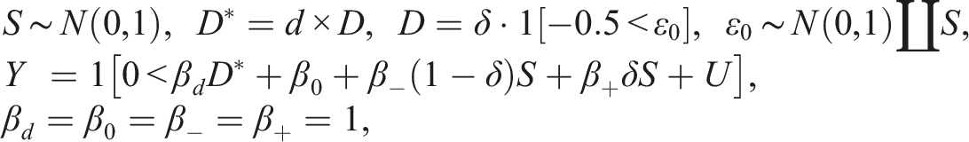
In RD, if $D$ is determined only by $S$ , then the RD is called a “sharp RD (SRD)”; if $D$ is determined by $(S, ε)$ where $ε$ is an error term, then the RD is called a “fuzzy RD (FRD).” In FRD, $D$ becomes endogenous/confounded if $ε$ affects $Y$ ; $D$ in SRD is always exogenous because no $ε$ appears. We have $D = 1 [S < c]$ in the above example, but we set $D$ in this paper either as $1 [c \leq S]$ for SRD or its “fuzzy version” for FRD. Also, we set $c = 0$ , which can be always arranged by redefining $S$ as $S - c$ (and multiplying by $- 1$ to reverse the inequality, if necessary). With the normalized $c = 0$ , define

δ \equiv 1 [0 \leq S];

δ = D

in SRD, and

δ

(\neq D)

is used as an instrument for endogenous

D

in FRD.

For practitioners not interested in the theoretical details, we present our main recommendation to do extrapolation in SRD and FRD for binary $Y$ with regressors

Z \equiv {\{δ, 1, (1 - δ) S, δ S\}}^{'} and \hat{W} \equiv {\{D, 1, (1 - δ) S, δ S, \hat{ε}\}}^{'};

(1)

\hat{ε}

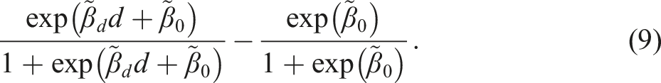
is introduced shortly. For SRD with

D = δ

, using a local sample with

| S | < h

for a chosen “bandwidth”

h > 0

, apply the logistic maximum likelihood estimator (MLE) of

Y

Z

to obtain the estimators

{\tilde{β}}_{d}

for

D

(= δ)

{\tilde{β}}_{0}

for

1

, and so on. Then the SRD effect of

D = d > 0

Y

(

d > 1

for extrapolation) relative to

D = 0

around

S = 0

\frac{\exp ({\tilde{β}}_{d} d + {\tilde{β}}_{0})}{1 + \exp ({\tilde{β}}_{d} d + {\tilde{β}}_{0})} - \frac{\exp ({\tilde{β}}_{0})}{1 + \exp ({\tilde{β}}_{0})} .

For FRD with $D \neq δ$ , still using the local sample, first, obtain the ordinary least squares estimator (OLS) $\hat{α}$ of $D$ on $Z$ to get the residual $\hat{ε} \equiv D - Z^{'} \hat{α}$ . Second, apply the local logistic MLE of $Y$ on $\hat{W}$ to obtain the estimators ${\hat{β}}_{d}$ for $D$ , ${\hat{β}}_{0}$ for $1$ , and so on. Third, find the effect of $D = d$ on $Y$ relative to $D = 0$ around $(\hat{ε} = 0, S = 0)$ with

\frac{\exp ({\hat{β}}_{d} d + {\hat{β}}_{0})}{1 + \exp ({\hat{β}}_{d} d + {\hat{β}}_{0})} - \frac{\exp ({\hat{β}}_{0})}{1 + \exp ({\hat{β}}_{0})} .

In the following, we introduce notation and some results in the RD literature to facilitate our discussion in Logistic Causal Model and Local MLE. Practitioners not keen on theoretical details may want skip the following to move on to Simulation Study and Income Effect on Being Evangelical for simulation and empirical studies.

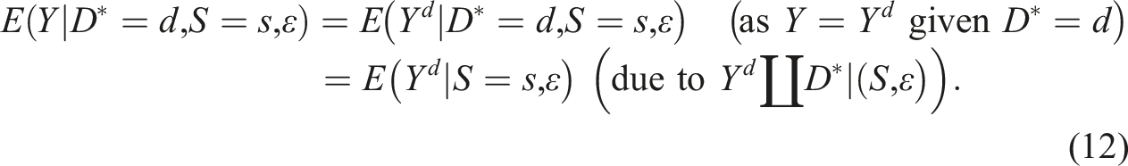
Let $(D^{0}, D^{1})$ be the potential binary treatments corresponding to $δ = 0, 1$ , and $(Y^{0}, Y^{1})$ be the potential versions corresponding to $D = 0, 1$ of the observed $Y$ ; for SRD, $D^{0} = 0$ and $D^{1} = 1$ due to $D = δ$ . Under $D^{1} \geq D^{0}$ , Hahn et al. (2001) showed

E (Y^{1} - Y^{0} | S = 0, D^{1} > D^{0}) = \frac{E (Y | 0^{+}) - E (Y | 0^{-})}{E (D | 0^{+}) - E (D | 0^{-})}

(2)

where

E (\cdot | 0^{+}) \equiv lim_{s ↓ 0} E (\cdot | S = s)

and

E (\cdot | 0^{-}) \equiv lim_{s ↑ 0} E (\cdot | S = s)

, which are the right- and left-limits at

s = 0

. The left-hand side of (2) is a “local average treatment effect” in Imbens and Angrist (1994), and those with

D^{1} > D^{0} \Leftrightarrow D^{1} - D^{0} = 1

are called “compliers” (Angrist et al., 1996). The right-hand side can be estimated with sample means around

S = 0

, or more generally, with a “local linear regression (LLR) estimator” or a local polynomial regression estimator.

Suppose we want to know the effect of an extrapolated treatment $D^{*}$ changing from $0$ to $d > 1$ ; since $D^{*} = d > 1$ is a counterfactual treatment, we use the notation $D^{*}$ to distinguish it from the actual binary treatment $D$ . An immediate answer based on (2) is a linear extrapolation:

\frac{E (Y | 0^{+}) - E (Y | 0^{-})}{E (D | 0^{+}) - E (D | 0^{-})} \times d = ‘effect of D = 1 ’ \times d .

(3)

However, despite that the effect should be a number in

[- 1, 1]

because

Y

is binary, (3) may not respect the bound, which is the problem with (3).

Linear extrapolation in (3) is simple, but it may not hold if the very fact of receiving the treatment per se shifts the intercept in $Y$ much while the treatment dose/intensity effect is relatively small, in which case increasing the dose has less than proportional effects. For instance, in the aforementioned food security study (for children), Collins et al. (2018) implemented the policy with $$ 0$ , $$ 30$ , and $$ 60$ monthly subsidies, where doubling $$ 30$ to $$ 60$ increased the policy effect far less than twice.

The issue of dose extrapolation is nowhere more critical than in toxicology, where a drug that has been tried only for some species or a group of humans (e.g., adults) has to be administered to other species or a different group of humans (e.g., infants); see Sharma and McNeil (2009) and references therein. An “allometric” scaling equation $P = α W^{β}$ is often employed for dose extrapolation, where $P$ is a metabolic rate, $α$ is a parameter, and $W$ is the body weight in kilogram with $β ≃ 0.75$ , because the metabolic rate slows down as the individual gets heavier due to the surface area (to lose the metabolic heat) increasing less than proportionally to the body weight. The point is that many things in life increase less than proportionately (e.g., $β < 1$ in $P = α W^{β}$ ), which is inevitable if there is an upper bound.

In a probability distribution, typically the majority of the probability mass is around the center of the distribution. This implies that increasing $P (Y = 1 | S)$ becomes harder at the tail areas of the latent continuous response, say $\tilde{Y}$ . This “probability-metric scaling” analogous to the allometric scaling is not taken into account in the linear extrapolation, as if increasing $P (Y = 1 | S)$ at a tail area of $\tilde{Y}$ is only as hard as it is at a central area. Essentially, this is why the bound $[- 1, 1]$ for $P (Y = 1 | S)$ is violated in finding the effect of an extrapolated treatment with (3).

A simple solution to the problem of violating the bound $[- 1, 1]$ is using a proper distribution for $P (Y = 1 | S)$ , for which we establish a “logistic causal model,” and propose a “local logistic MLE.” We then make the following points. First, the local logistic MLE always respects the $[- 1, 1]$ bound. Second, for the usual treatment level $d = 1$ , the MLE gives almost the same effect estimate as the popular LLR does in RD, and when $d > 1$ , the MLE still gives estimates in $[- 1, 1]$ , which is not the case for LLR. Third, although we use logistic distribution, normal distribution may be adopted instead. These points are demonstrated through simulation and empirical studies.

We are not the first to consider local MLE’s for RD. Local logistic MLE for RD appeared in Berk & de Leeuw, 1999; Berk & Rauma, 1983. Koch and Racine (2016) applied local multinomial logit to SRD, which includes local logistic MLE as a special case. Xu (2017) examined ordered/categorical responses including binary $Y$ as a special case for SRD; the proposed estimator takes a form of probability difference. Xu (2017) noted that his method can be extended to FRD by dividing the probability difference for $Y$ by the corresponding difference for $D$ , but such a division may not fall in $[- 1, 1]$ in extrapolating the treatment. Extrapolating treatment bears resemblance to the “external validity” issue in RD (Angrist & Rokkanen, 2015; Dong & Lewbel, 2015), yet these studies differ from this paper because they are about extending the RD identification range on $S$ from the cutoff, not for extrapolating the treatment.

In addition to this introductory section, there are four more sections in the remainder of this paper. The next section introduces a causal model and the local logistic MLE for SRD and FRD, which is then followed by two sections on simulation and empirical studies. The last section concludes this paper.

Logistic Causal Model and Local MLE

To prevent confusion, we make it clear how the counterfactual extrapolated treatment $D^{*}$ is related to the original binary treatment D:

D^{*} = d \times D (\Rightarrow D^{*} = d \times δ for SRD) .

This includes an implicit assumption for FRD that the complier group

(D^{1} = 1, D^{0} = 0)

does not change when

d

does. That is, those who take the treatment when

D = 0, 1

still take it when the treatment is

D^{*} = 0, d > 1

, and those who do not take the treatment when

D = 0, 1

still do not take it when the treatment is

D^{*} = 0, d > 1

Since $D^{*}$ is just a constant $(d)$ times $D$ , (in-)dependence between $D$ and other random variables still hold for $D^{*}$ . For instance, letting “ $A ∐ B | C$ ” stand for the independence between $A$ and $B$ given $C$ , we have $D ∐ Y^{0} | S \Leftrightarrow D^{*} ∐ Y^{0} | S$ . With these $D^{*}$ and $D$ , we address SRD first in this section, and then FRD.

Logistic Causal Model for SRD

Suppose that a “marginal structural logistic model” holds for the potential outcome $Y^{d}$ for $D^{*} = d :$

E (Y^{d} | S = s) = \frac{\exp \{β_{d} d + m (s)\}}{1 + \exp \{β_{d} d + m (s)\}} for all d \geq 0

(4)

where

β_{d}

is the treatment effect, and

m (S)

is an unknown function that is continuous at

0

. The term “marginal” in causal analysis refers to the fact that many

Y^{d}

’s indexed by

d

are jointly considered, and

Y^{d}

is just one of them. The potential treatment level

d

Y^{d}

does not have to be compatible with

S = s

; for example, (4) with

(d = 1, s < 0)

is entertained for SRD with the treatment

δ \equiv 1 [0 \leq S]

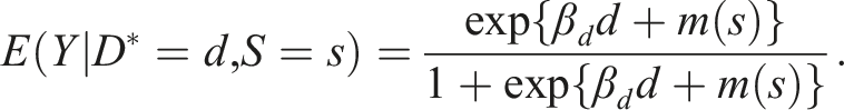
Consider an exogenous $D^{*}$ in the sense $Y^{d} ∐ D^{*} | S (\Leftrightarrow Y^{d} ∐ D | S)$ which is called “selection on observables”; $S$ is the observable. For a compatible $(D^{*} = d, S = s),$

\begin{aligned} E (Y | D^{*} = d, S = s) = E (Y^{d} | D^{*} = d, S = s) (as Y = Y^{d} given D^{*} = d) \\ = E (Y^{d} | S = s) (due to Y^{d} ∐ D^{*} | S) . \end{aligned}

(5)

Substitute (4) into the

E (Y^{d} | S = s)

in (5) to get

E (Y {| D}^{*} = d, S = s) = \frac{\exp \{β_{d} d + m (s)\}}{1 + \exp \{β_{d} d + m (s)\}} .

Omitting “

= d

” and “

= s

” in “

D^{*} = d

” and “

S = s

” gives

E (Y {| D}^{*}, S) = \frac{\exp \{β_{d} D^{*} + m (S)\}}{1 + \exp \{β_{d} D^{*} + m (S)\}} .

(6)

Because

d

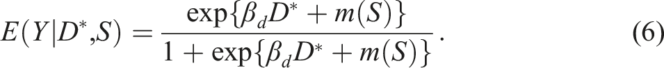
in (4) is just a constant, (4) does not specify how

D^{*} = d \times D

is related to

Y^{d}

and

S

; it is (5) that specifies the relationship as the exogeneity of

D^{*} = d \times D

for

Y^{d}

given

S

. We can then use (6) and observations on

(D, Y, S)

to estimate

β_{d}

, to which we turn next.

Local Logistic MLE for SRD

Slightly differently from the regressors in (1), define

X \equiv {\{D, 1, (1 - δ) S, δ S\}}^{'} .

(7)

Replacing

m (S)

in (6) with a “linear spline”

β_{0} + β_{-} (1 - δ) S + β_{+} δ S

gives

E (Y | D, S) = \frac{\exp (X^{'} β_{x})}{1 + \exp (X^{'} β_{x})} where β_{x} \equiv {(β_{d}, β_{0}, β_{-}, β_{+})}^{'} .

(8)

Then we can do logistic MLE of

Y

X

with the local sample satisfying

Q = 1

, where

Q \equiv 1 [| S | < h]

for a chosen small bandwidth

h > 0

In (8), $m (S)$ that is supposed to be continuous at $S = 0$ is approximated by a piecewise linear function $β_{0} + β_{-} (1 - δ) S + β_{+} δ S$ with $m (0) = β_{0}$ , which allows different slopes around $0$ : $β_{-}$ on the negative side, and $β_{+}$ on the positive side. Since $h \to 0^{+}$ as the sample size $N \to \infty$ , this approximation of $m (S)$ is innocuous.

Denoting the local logistic MLE for $β_{x}$ as ${({\tilde{β}}_{d}, {\tilde{β}}_{0}, {\tilde{β}}_{-}, {\tilde{β}}_{+})}^{'}$ , the mean treatment effect for $D^{*} = d$ relative to $D^{*} = 0$ on the subpopulation $S ≃ 0$ can be estimated with

\frac{\exp ({\tilde{β}}_{d} d + {\tilde{β}}_{0})}{1 + \exp ({\tilde{β}}_{d} d + {\tilde{β}}_{0})} - \frac{\exp ({\tilde{β}}_{0})}{1 + \exp ({\tilde{β}}_{0})} .

(9)

This was already presented in Introduction.

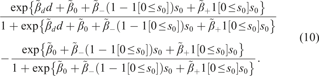
More generally, to extrapolate $D$ to $D^{*} = d \times D$ on some value of $S$ other than $0$ , say $s_{0}$ , we may use

\begin{array}{l} \frac{\exp \{{\tilde{β}}_{d} d + {\tilde{β}}_{0} + {\tilde{β}}_{-} (1 - 1 [0 \leq s_{0}]) s_{0} + {\tilde{β}}_{+} 1 [0 \leq s_{0}] s_{0}\}}{1 + \exp \{{\tilde{β}}_{d} d + {\tilde{β}}_{0} + {\tilde{β}}_{-} (1 - 1 [0 \leq s_{0}]) s_{0} + {\tilde{β}}_{+} 1 [0 \leq s_{0}] s_{0}\}} \\ - \frac{\exp \{{\tilde{β}}_{0} + {\tilde{β}}_{-} (1 - 1 [0 \leq s_{0}]) s_{0} + {\tilde{β}}_{+} 1 [0 \leq s_{0}] s_{0}\}}{1 + \exp \{{\tilde{β}}_{0} + {\tilde{β}}_{-} (1 - 1 [0 \leq s_{0}]) s_{0} + {\tilde{β}}_{+} 1 [0 \leq s_{0}] s_{0}\}} . \end{array}

(10)

For this to work, we need three main conditions to hold:

(i): the logistic assumption (4);

(ii): the selection-on-observable assumption (5);

(iii): $m (S) = β_{0} + β_{-} (1 - δ) S + β_{+} δ S$ .

s_{0}

differs much from

0

, then we may have to use a more extensive specification for

m (S)

, so that the unknown functional form of

m (S)

can be captured better.

A few remarks are in order. First, the asymptotic inference can be done with the usual logistic MLE variance estimator using only the local sample. Second, instead of (8), we may set $E (Y | D, S) = Φ (X^{'} β_{x})$ to do local probit MLE, where $Φ$ is the $N (0,1)$ distribution function. Third, in choosing $h$ , Imbens and Kalyanaraman (2012) and Calonico et al. (2014) proposed optimal bandwidths for RD, but they do not necessarily work well in practice, which was pointed out by Card et al. (2017) for “regression kink” design. In practice, one may use the simple “rule-of-thumb” bandwidth $h_{r u l e} \equiv S D (S) N^{- 1 / 5}$ as a benchmark, and report estimates for different bandwidths around the benchmark, such as $0.5 \times h_{r u l e}$ or $2 \times h_{r u l e}$ .

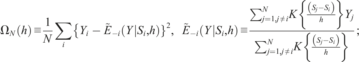
Alternatively to $h_{r u l e}$ , one may use the $h$ minimizing

Ω_{N} (h) \equiv \frac{1}{N} \sum_{i} {Y_{i} - {\tilde{E}}_{- i} (Y {| S}_{i}, h)}^{2}, {\tilde{E}}_{- i} (Y {| S}_{i}, h) \equiv \frac{\sum_{j = 1, j \neq i}^{N} K \{\frac{(S_{j} - S_{i})}{h}\} Y_{j}}{\sum_{j = 1, j \neq i}^{N} K \{\frac{(S_{j} - S_{i})}{h}\}};

K (\cdot)

is a “kernel function” such as the

N (0,1)

density, and this

h

-choosing scheme is called “cross-validation (CV).” In

Ω_{N} (h)

{\tilde{E}}_{- i} (Y {| S}_{i}, h)

is a “leave-one-out” kernel nonparametric estimator for

E (Y | S = S_{i})

;

Ω_{N} (h)

tends to behave well, being nearly convex in

h

. Appendix A provides more discussion on choosing

h

with CV.

Logistic Causal Model for FRD

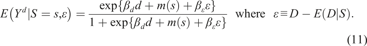
Suppose a “marginal structural logistic model augmented by $ε$ ” holds for $Y^{d}$ : for a parameter $β_{ε},$

E (Y^{d} | S = s, ε) = \frac{\exp \{β_{d} d + m (s) + β_{ε} ε\}}{1 + \exp \{β_{d} d + m (s) + β_{ε} ε\}} where ε \equiv D - E (D | S) .

(11)

Consider an endogenous

D^{*}

in the sense

Y^{d} ∐ D^{*} | (S, ε)

, which is “selection on unobservables”;

ε

is the unobservable. Although the mean independence (5) of

Y^{d}

from

D^{*}

given only

S

no more holds, it holds given

(S, ε)

Analogous to (5) is that

\begin{aligned} E (Y {| D}^{*} = d, S = s, ε) = E (Y^{d} {| D}^{*} = d, S = s, ε) (as Y = Y^{d} given D^{*} = d) \\ = E (Y^{d} | S = s, ε) (due to Y^{d} ∐ D^{*} | (S, ε)) . \end{aligned}

(12)

Analogously to (4) to (6), we also obtain

E (Y {| D}^{*}, S, ε) = \frac{\exp \{β_{d} D^{*} + m (S) + β_{ε} ε\}}{1 + \exp \{β_{d} D^{*} + m (S) + β_{ε} ε\}} .

(13)

D = E (D | S) + ε

, the “

S

-part”

E (D | S)

cannot be the source for the endogeneity of

D

. Hence the only way for

D

to be endogenous is through the part of

D

other than

E (D | S)

, which is

ε

As will be seen shortly, we find the treatment effect at $(S = 0, ε = 0)$ . Conditioning on $S = 0$ is no surprise because the identified treatment effect in RD is at the cutoff. What is notable is conditioning on $ε \equiv D - E (D | S) = 0$ , which is equivalent to

‘ D determined solely by S ’ \Leftrightarrow D = δ \Leftrightarrow (D^{1} = 1, D^{0} = 0) (compliers) .

That is,

ε = 0

ensures that the treatment effect on the compliers is identified as in

E (Y^{1} - Y^{0} | S = 0, D^{1} > D^{0})

of (2), despite that the ratio form in the right-hand side of (2) is not used. We explain the difference between our

ε

-controlling approach in (11) to (13) and the ratio-based approach in (2) in the remainder of this subsection, using simple linear models.

Consider two models for $Y$ and endogenous $D$ : with some $α$ and $β$ parameters,

D = α_{0} + α_{δ} δ + ε and Y = β_{0} + β_{d} D + U .

Substitute the

D

model into the

Y

model to obtain

Y = β_{0} + β_{d} (α_{0} + α_{δ} δ + ε) + U = (β_{0} + β_{d} α_{0}) + β_{d} α_{δ} δ + (β_{d} ε + U) .

An “indirect” way to find the treatment effect $β_{d}$ is a two-stage ratio estimator: do the OLS of $D$ on $(1, δ)$ to get the slope ${\hat{α}}_{δ}$ and the OLS of $Y$ on $(1, δ)$ to get the slope $\hat{β_{d} α_{δ}}$ for the last display, and then use the ratio $\hat{β_{d} α_{δ}} / {\hat{α}}_{δ}$ as an estimator for $β_{d}$ . This ratio is in essence the same as the ratio in (2), revealing that the ratio in (2) is an indirect approach.

In contrast to the indirect approach, a “direct” way to find $β_{d}$ is applying instrumental variable estimator (IVE) for $Y$ on $(1, D)$ with $δ$ as an instrument for $D$ . This IVE is the same as the OLS of $Y$ on $(1, D, \hat{ε})$ with $\hat{ε}$ being the OLS residual of $D$ ; see, for example, Lee (2012). The extra regressor $\hat{ε}$ is called a “control function,” whose role is to remove the $D$ endogeneity.

In short, the $ε$ -controlling approach in (11) to (13) is a direct approach to find the left-hand side of (2), whereas the right-hand side ratio of (2) is an indirect approach. Appendix B explains the indirect ratio-based approach for $D^{*}$ in detail, as it is the dominant conventional approach to find the FRD effect of $D$ at the cutoff, although it is not well suited for $D^{*}$ when $Y$ is binary.

Local Logistic MLE for FRD

With $\hat{W} \equiv {D, 1, (1 - δ) S, δ S, \hat{ε}}^{'}$ in (1), define

W \equiv {(X^{'}, ε)}^{'} = {\{D, 1, (1 - δ) S, δ S, ε\}}^{'} .

Replacing

m (S)

with the linear spline

β_{0} + β_{-} (1 - δ) S + β_{+} δ S

in (13) renders

E (Y | D, S, ε) = \frac{\exp (W^{'} β_{w})}{1 + \exp (W^{'} β_{w})}, β_{w} \equiv {(β_{d}, β_{0}, β_{-}, β_{+}, β_{ε})}^{'} = {(β_{x}^{'}, β_{ε})}^{'} .

(14)

Our proposal for FRD is a two-stage procedure using the local

Q = 1

observations: the first stage is the local OLS of

D

Z \equiv {δ, 1, (1 - δ) S, δ S}^{'}

(which depends only on

S

) to obtain the OLS

\hat{α}

and the residual

\hat{ε} \equiv D - Z^{'} \hat{α}

, and the second stage is the local logistic MLE of

Y

\hat{W} \equiv {D, 1, (1 - δ) S, δ S, \hat{ε}}^{'}

. Although

ε

was defined as

D - E (D | S)

in (11), we set

ε = D - Z^{'} α

, whose justification is shown shortly below.

Denoting the local logistic MLE for $β_{w}$ as ${\hat{β}}_{w} \equiv {({\hat{β}}_{d}, {\hat{β}}_{0}, {\hat{β}}_{-}, {\hat{β}}_{+}, {\hat{β}}_{ε})}^{'}$ , the asymptotic inference can be done with the usual logistic MLE asymptotic variance, and “ $H_{0} : β_{ε} = 0$ (i.e., $D$ exogeneity)” can be tested with ${\hat{β}}_{ε}$ . Although there is the first-stage error $\hat{α} - α$ affecting the second stage, its influence can be ignored under the $H_{0}$ . Just in case, Appendix D provides an asymptotic variance estimator fully accounting for the first-stage error. Alternatively, we may use bootstrap, which is simpler.

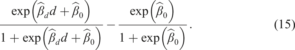
Analogously to (9), the mean effect of $D^{*}$ changing from $0$ to $d$ at $(ε = 0, S = 0)$ can be estimated with

\frac{\exp ({\hat{β}}_{d} d + {\hat{β}}_{0})}{1 + \exp ({\hat{β}}_{d} d + {\hat{β}}_{0})} - \frac{\exp ({\hat{β}}_{0})}{1 + \exp ({\hat{β}}_{0})} .

(15)

This was already presented in Introduction.

The basis for using $\hat{ε} \equiv D - Z^{'} \hat{α}$ as a control function has two parts. The first part is an equivalence: for an unknown function $m_{D} (S)$ continuous at $0,$

E (D | S) = α_{δ} δ + m_{D} (S) \Leftrightarrow α_{δ} \equiv E (D | 0^{+}) - E (D | 0^{-})

(16)

which is proven in Appendix C. Then, replacing

m_{D} (S)

with a linear spline

α_{0} + α_{-} (1 - δ) S + α_{+} δ S

gives

E (D | S) = Z^{'} α

, where

α \equiv {(α_{δ}, α_{0}, α_{-}, α_{+})}^{'}

. The second part is the fact that the IVE for the linear model

Y = β_{d} D + β_{0} + β_{-} (1 - δ) S + β_{+} δ S + e r r o r

(17)

with

D

instrumented by

δ

is equal to the

(β_{d}, β_{0}, β_{-}, β_{+})

part of the OLS for

Y = β_{d} D + β_{0} + β_{-} (1 - δ) S + β_{+} δ S + β_{ε} \hat{ε} + e r r o r^{'} .

(18)

The local logistic MLE with

\hat{ε}

to account for the

D

endogeneity differs from the IVE for LLR of (17) only in that the

(0,1)

-bounded logistic function is used instead of the linear model, which makes a good sense for binary

Y

To extrapolate $D$ to $D^{*} = d \times D$ on some value of $S$ other than $0$ , say $s_{0}$ , we may use (10) with $\tilde{β}$ replaced by $\hat{β}$ . For this to work, we need five main conditions to hold:

(i): the logistic assumption (11);

(ii): the selection-on-unobservable assumption (12);

(iii): $m (S) = β_{0} + β_{-} (1 - δ) S + β_{+} δ S$ ;

(iv): (16) that $E (D | S)$ has a break at $S = 0$ ;

(v): $m_{D} (S) = α_{0} + α_{-} (1 - δ) S + α_{+} δ S$ in (16).

Compared with the three main conditions for SRD extrapolation with

s_{0}

right after (10), (iv) and (v) are extra, which may be viewed as conditions for the denominator of (2): (iv) ensures that the denominator is not zero, and (v) ensures that

α_{δ}

is estimable by the OLS of

D

Z

. If

s_{0}

differs much from

0

, then we may have to use more extensive specifications for

m (S)

and

m_{D} (S)

, so that the unknown functional forms of

m (S)

and

m_{D} (S)

can be better captured.

Simulation Study

This section presents a simulation study to demonstrate three points. First, for $d = 1$ , local logistic MLE (“MLE” in the remainder of this section) performs almost the same as LLR estimator does. Second, for $d = 2, 4$ , MLE does much better than LLR. Third, MLE performs well even if probit is used instead of logit. If we want to distinguish MLE’s for exogenous and endogenous $D$ , we write “MLEex” and “MLEcf,” respectively.

Our simulation designs are as follows:

\begin{array}{l} S \sim N (0, 1), D^{*} = d \times D, D = δ \cdot 1 [- 0.5 < ε_{0}], ε_{0} \sim N (0, 1) ∐ S, \\ Y = 1 [0 < β_{d} D^{*} + β_{0} + β_{-} (1 - δ) S + β_{+} δ S + U], \\ β_{d} = β_{0} = β_{-} = β_{+} = 1, \end{array}

(i): $U \sim L o g i s t i c ∐ (S, ε_{0})$ , so that $D$ is exogenous (for Table 1 below);

(ii): $U \sim N (0, {1.8}^{2}) ∐ (S, ε_{0})$ , so that $D$ is exogenous (Table 2);

(iii): $U \sim N (0, {1.8}^{2}) ∐ S$ , $C O R (U, ε_{0}) = \sqrt{0.5}$ so that $D$ is endogenous (Table 3).

Table 1.

Effect and Bias Under Logistic Error and Exogenous $D$ .

$N = 3000$ and $h = N^{- 1 / 5}$
True effect	LLR (bias)	MLEex (bias)	MLEcf (bias)
0.15 $(d = 1)$	0.15 (0.003)	0.15 (0.012)	0.14 (0.037)
0.22 $(d = 2)$	0.30 (0.36)	0.22 (0.028)	0.20 (0.11)
0.26 $(d = 4)$	0.60 (1.3)	0.26 (0.022)	0.22 (0.15)
${\tilde{β}}_{d}$ , ${\hat{β}}_{d}$ (sd-asy, sd)	—	1.0 (0.35, 0.35)	1.0 (0.70, 0.70)
Reject exogeneity	—	—	0.051 (0.045)
$N = 6000$ and $h = N^{- 1 / 5}$
0.15 $(d = 1)$	0.15 (0.001)	0.15 (0.005)	0.15 (0.024)
0.22 $(d = 2)$	0.30 (0.35)	0.22 (0.014)	0.21 (0.068)
0.26 $(d = 4)$	0.60 (1.3)	0.26 (0.011)	0.24 (0.079)
${\tilde{β}}_{d}$ , ${\hat{β}}_{d}$ (sd-asy, sd)	—	1.0 (0.26, 0.26)	1.0 (0.52, 0.53)
Reject exogeneity	—	—	0.051 (0.048)
$N = 3000$ and $h = 2.5 N^{- 1 / 5}$
0.15 $(d = 1)$	0.15 (0.000)	0.15 (0.001)	0.15 (0.017)
0.22 $(d = 2)$	0.30 (0.35)	0.22 (0.010)	0.21 (0.047)
0.26 $(d = 4)$	0.60 (1.3)	0.26 (0.007)	0.25 (0.049)
${\tilde{β}}_{d}$ , ${\hat{β}}_{d}$ (sd-asy, sd)	—	1.0 (0.23, 0.23)	1.0 (0.44, 0.44)
Reject exogeneity	—	—	0.049 (0.048)

Bias: $| estimated effect−true effect | / | true effect |$ ; sd-asy: avg. SD with asy. var.; sd: SD in simulation; reject exogeneity: rejection proportion with sd-asy (proportion with sd-asy ignoring $\hat{ε} - ε$ ).

Table 2.

Effect and Bias Under Normal Error and Exogenous $D .$

$N = 3000$ and $h = N^{- 1 / 5}$
True effect	LLR (bias)	MLEex (bias)	MLEcf (bias)
0.16 $(d = 1)$	0.16 (0.003)	0.16 (0.004)	0.15 (0.037)
0.24 $(d = 2)$	0.32 (0.29)	0.23 (0.052)	0.21 (0.14)
0.29 $(d = 4)$	0.62 (1.2)	0.28 (0.041)	0.24 (0.17)
${\tilde{β}}_{d}$ , ${\hat{β}}_{d}$ (sd-asy, sd)	—	1.0 (0.33, 0.33)	1.0 (0.68, 0.67)
Reject exogeneity	—	—	0.045 (0.041)
$N = 6000$ and $h = N^{- 1 / 5}$
0.16 $(d = 1)$	0.16 (0.007)	0.16 (0.005)	0.15 (0.014)
0.24 $(d = 2)$	0.31 (0.30)	0.23 (0.037)	0.22 (0.087)
0.29 $(d = 4)$	0.63 (1.2)	0.28 (0.027)	0.26 (0.090)
${\tilde{β}}_{d}$ , ${\hat{β}}_{d}$ (sd-asy, sd)	—	0.99 (0.25, 0.25)	1.0 (0.50, 0.50)
Reject exogeneity	—	—	0.049 (0.045)
$N = 3000$ and $h = 2.5 N^{- 1 / 5}$
0.16 $(d = 1)$	0.16 (0.002)	0.16 (0.015)	0.15 (0.014)
0.24 $(d = 2)$	0.31 (0.30)	0.24 (0.028)	0.22 (0.074)
0.29 $(d = 4)$	0.63 (1.2)	0.28 (0.022)	0.27 (0.069)
${\tilde{β}}_{d}$ , ${\hat{β}}_{d}$ (sd-asy, sd)	—	1.0 (0.22, 0.22)	1.0 (0.43, 0.43)
Reject exogeneity	—	—	0.047 (0.045)

Table 3.

Effect and Bias Under Normal Error and Endogenous $D$ .

$N = 3000$ and $h = N^{- 1 / 5}$
True effect	LLR (bias)	MLEex (bias)	MLEcf (bias)
0.16 $(d = 1)$	0.097 (0.38)	0.36 (1.3)	0.21 (0.35)
0.24 $(d = 2)$	0.19 (0.20)	0.38 (0.58)	0.26 (0.075)
0.29 $(d = 4)$	0.39 (0.35)	0.38 (0.34)	0.28 (0.036)
${\tilde{β}}_{d}$ , ${\hat{β}}_{d}$ (sd-asy, sd)	—	3.6 (0.51, 0.56)	1.7 (0.85, 0.83)
Reject exogeneity	—	—	0.78 (0.76)
$N = 6000$ and $h = N^{- 1 / 5}$
0.16 $(d = 1)$	0.10 (0.36)	0.36 (1.3)	0.22 (0.38)
0.24 $(d = 2)$	0.20 (0.17)	0.38 (0.57)	0.27 (0.11)
0.29 $(d = 4)$	0.40 (0.40)	0.38 (0.33)	0.29 (0.004)
${\tilde{β}}_{d}$ , ${\hat{β}}_{d}$ (sd-asy, sd)	—	3.5 (0.37, 0.41)	1.74 (0.63, 0.64)
Reject Exogeneity	—	—	0.95 (0.94)
$N = 3000$ and $h = 2.5 N^{- 1 / 5}$
0.16 $(d = 1)$	0.10 (0.34)	0.36 (1.3)	0.22 (0.43)
0.24 $(d = 2)$	0.21 (0.15)	0.38 (0.56)	0.27 (0.13)
0.29 $(d = 4)$	0.41 (0.43)	0.38 (0.32)	0.29 (0.006)
${\tilde{β}}_{d}$ , ${\hat{β}}_{d}$ (sd-asy, sd)	—	3.6 (0.34, 0.38)	1.8 (0.54, 0.55)
Reject Exogeneity	—	—	0.99 (0.99)

With $N (0, {1.8}^{2})$ , the normal distribution has $S D = 1.8$ as the logistic distribution does. Although the “structural form error” $ε_{0}$ in $δ \cdot 1 [- 0.5 < ε_{0}]$ causes the endogeneity of $D$ unless $ε_{0} ∐ U$ , $ε_{0}$ differs from the “reduced form error” $ε \equiv D - E (D | S)$ .

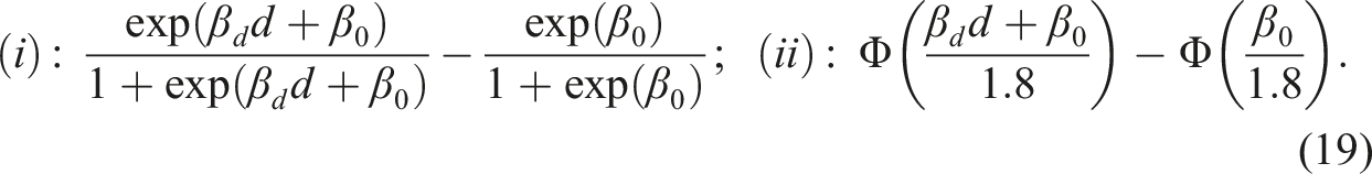
We use two bandwidths: with $S D (S) = 1$ , the rule-of-thumb bandwidth $N^{- 1 / 5}$ and $2.5 \times N^{- 1 / 5}$ ; CV takes too much time to implement in simulation. The sample size is $N = 3000, 6000$ with the simulation repetition $10,000$ . The sample size may look large, but the actual size used for estimation is much smaller due to $Q \equiv 1 [| S | < h]$ . For instance, $N^{- 1 / 5}$ equals $0.202$ when $N = 3000$ , and consequently $E (Q)$ equals $0.16$ : only $3000 \times 0.16 = 480$ observations are used for estimation. The true effect of $D^{*}$ changing from $0$ to $d = 1, 2, 4$ given $(ε_{0} = 0, S = 0)$ is, depending on $U$ logistic or $N (0, {1.8}^{2}),$

(i) : \frac{\exp (β_{d} d + β_{0})}{1 + \exp (β_{d} d + β_{0})} - \frac{\exp (β_{0})}{1 + \exp (β_{0})}; (i i) : Φ (\frac{β_{d} d + β_{0}}{1.8}) - Φ (\frac{β_{0}}{1.8}) .

(19)

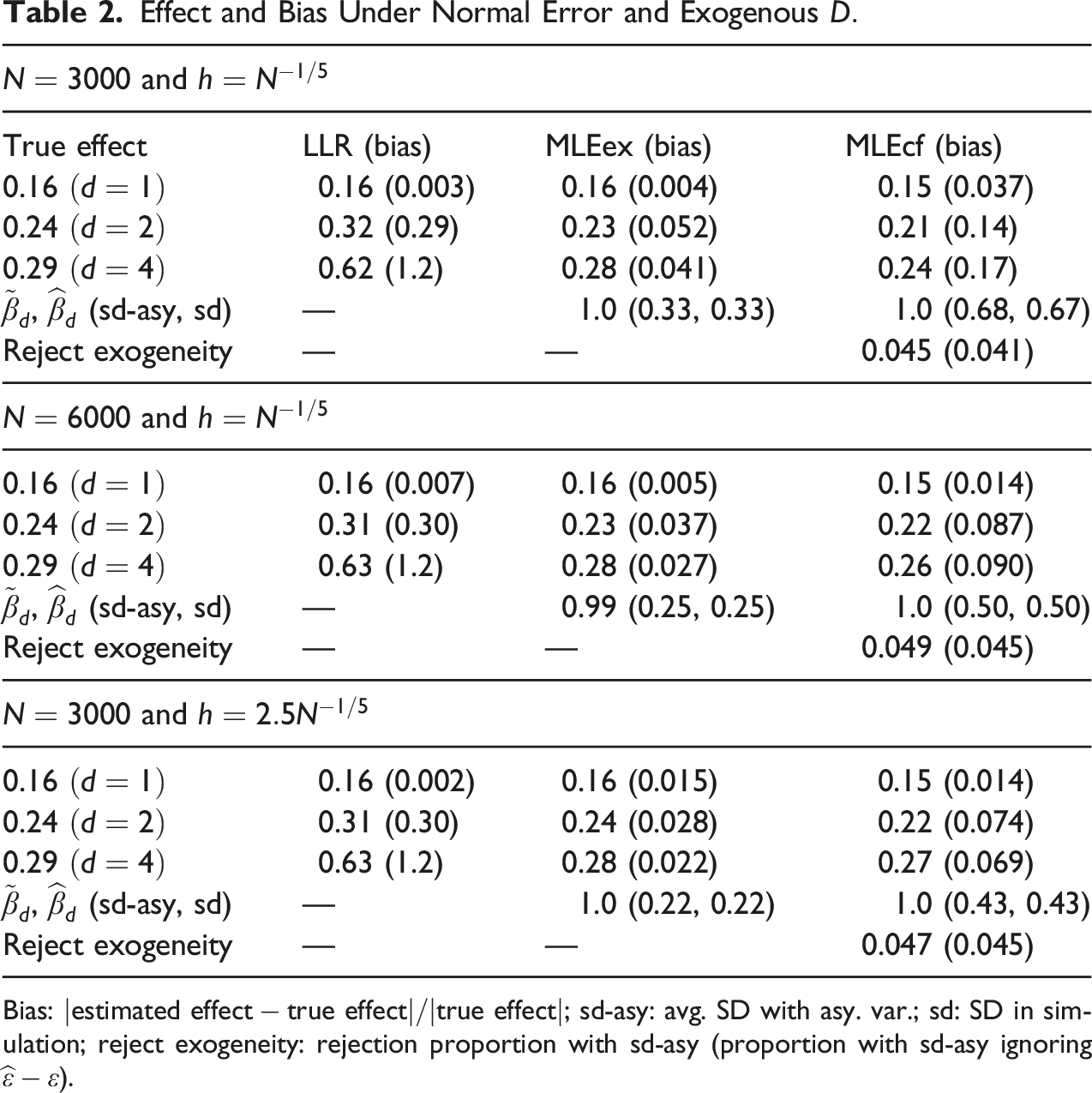
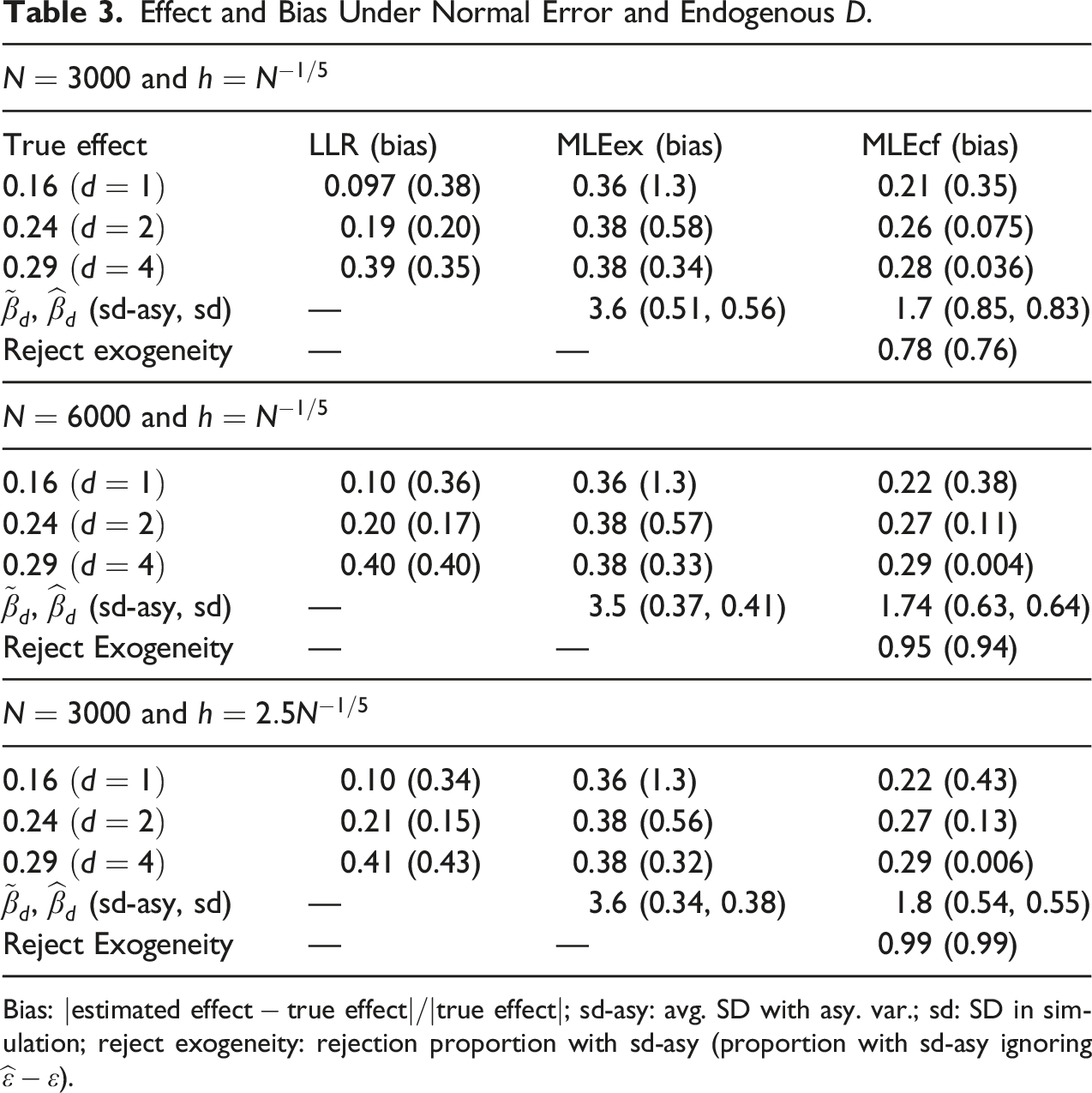
In Table 1, the upper panel is for

N = 3000

and

h = N^{- 1 / 5}

, the middle panel is for

N = 6000

and

h = N^{- 1 / 5}

, and the lower panel is for

N = 3000

and

h = 2.5 N^{- 1 / 5}

. In each panel, the first column shows the true effect (19) for

d = 1, 2, 4

; the second column shows the LLR effect using the linear extrapolation as in (3), and the (relative) bias

|(LLR - true) / true|

(e.g., the LLR effect

0.30

for

d = 2

has the bias

0.36 ≃ |(0.30 - 0.22) / 0.22|

; the third column shows (9) using MLEex, and its bias; and the fourth column shows (15) using MLEcf, and its bias. The row “

{\tilde{β}}_{d}

{\hat{β}}_{d}

(sd-asy, sd)” presents the averaged

{\tilde{β}}_{d}

{\hat{β}}_{d}

, the averaged SD using the asymptotic variance estimator (sd-asy), and the actual SD in the simulation repetitions (sd). The row “reject exogeneity” is the rejection rate for “

H_{0}

D

is exogenous” using the t-value of the slope of

\hat{ε}

and the critical values

\pm 1.96

. The test is done with the asymptotic variance formula in Appendix D that takes the first-stage error

\hat{ε} - ε

into account first, and then with the asymptotic variance ignoring

\hat{ε} - ε

whose rejection rate is in (

\cdot

In Table 1 with logistic $U$ and exogenous $D$ , the overall performance ranking in terms of the sum of the three biases for $d = 1, 2, 4$ is, with “ $≻$ ” for “better than”,

MLEex ≻ MLEcf ≻ LLR.

(20)

LLR does best for

d = 1

, and the MLE’s do almost as well for

d = 1

. For

d = 2, 4

, however, LLR is highly biased. Comparing the sd-asy’s to the actual simulation SD’s, the asymptotic SD formulas work well for the MLE’s. The false rejection rates are all close to

5 %

to validate the exogeneity test with or without taking into account

\hat{ε} - ε

. Increasing

h

2.5

times in the bottom panel makes little difference.

In Table 2, $U$ is normal with $D$ still exogenous. Although the distribution of $U$ changes, still all points made for Table 1 hold for Table 2, including the ranking in (20).

In Table 3, $U$ is still normal, but $D$ is endogenous. Although no estimator works particularly well because binary endogenous regressor with binary response is particularly difficult to deal with (see, e.g., Lee, 2012, and Clarke & Windmeijer, 2012), still MLEcf works much better than LLR and MLEex, and the performance ranking in terms of the sum of the three biases is

MLEcf ≻ LLR ≻ MLEex.

(21)

The

D

-exogeneity is easily rejected, with the rejection rate

76 %

or higher.

In summary, comparing Table 1, Table 2 and Table 3, MLEcf renders the most robust performance all around, although MLEex does better when $D$ is exogenous. The asymptotic SD formula of MLEcf works well, almost equaling the actual SD, and its $D$ -exogeneity test also works reliably even when the first-stage error $\hat{ε} - ε$ is ignored. Hence, a sensible scenario to follow in practice for FRD is applying MLEcf first to test for $D$ exogeneity. If rejected, stick to MLEcf; otherwise, use MLEex.

Income Effect on Being Evangelical

This section provides an empirical illustration using the same data as used in Buser (2015), although Buser (2015) did not examine the issue of treatment dose extrapolation. This section will confirm that both LLR and local logistic MLE effects are almost the same for the original treatment $D = 1$ , but they differ much for extrapolated treatment doses. This section will also demonstrate that the bound $[- 1, 1]$ can be violated for a high treatment dose.

According to Buser (2015), Ecuador is a highly Catholic country: $76 %$ are Catholic, and $10 %$ belong to the Evangelical Christian denomination which is non-Catholic. But being Evangelical is more demanding than being Catholic in terms of money and time, because Evangelical churches are highly integrated and more participative, and they also require a tithe. This financial commitment deters the poor from becoming Evangelical even if they like Evangelism. Hence, more income may induce more religious and poor people to become Evangelical $(Y)$ .

A RD setup occurred due to a government cash subsidy program $D$ giving $$ 35$ per month to the poorest $40 %$ households based on a wealth index $S$ . Although $$ 35$ sounds small, that is not the case because $$ 35$ is about $12 %$ of the monthly total expenditure. Location-normalizing $S$ and then multiplying $S$ by $- 1$ , we have $δ = 1 [0 \leq S]$ . Since the sampling was done already only from the individuals within $0.3 \times S D (S)$ distance from the cutoff, Buser (2015) used all data without selecting any subsample, and we will do the same; that is, no issue of choosing $h$ arises in this empirical analysis.

Buser (2015) found significantly positive effects of $D$ on $Y$ , and noted that the effects come mostly from the above-average religious individuals. In the survey data with $N = 2645$ , there is a religiosity variable $R \in [0, 10]$ with $10$ being the most religious; the average is $6.82$ . We thus use the above-average-religiosity subsample with $R \geq 7$ and $N = 1480$ . We also use the most religious group with $R = 10$ with $N = 482$ . See Buser (2015) for the details on the data, as well as the usual RD plots visually demonstrating breaks in $E (D | S)$ and $E (Y | S)$ . As in the simulation section, we examine treatment dose extrapolation $D^{*} = 2, 4$ from the original $D = 1$ . Buser (2015) used polynomial functions for $m (S)$ , but we stick to the linear spline. Also, Buser (2015) controlled covariates sometimes, which we do not do though, because controlling covariates is not essential in RD.

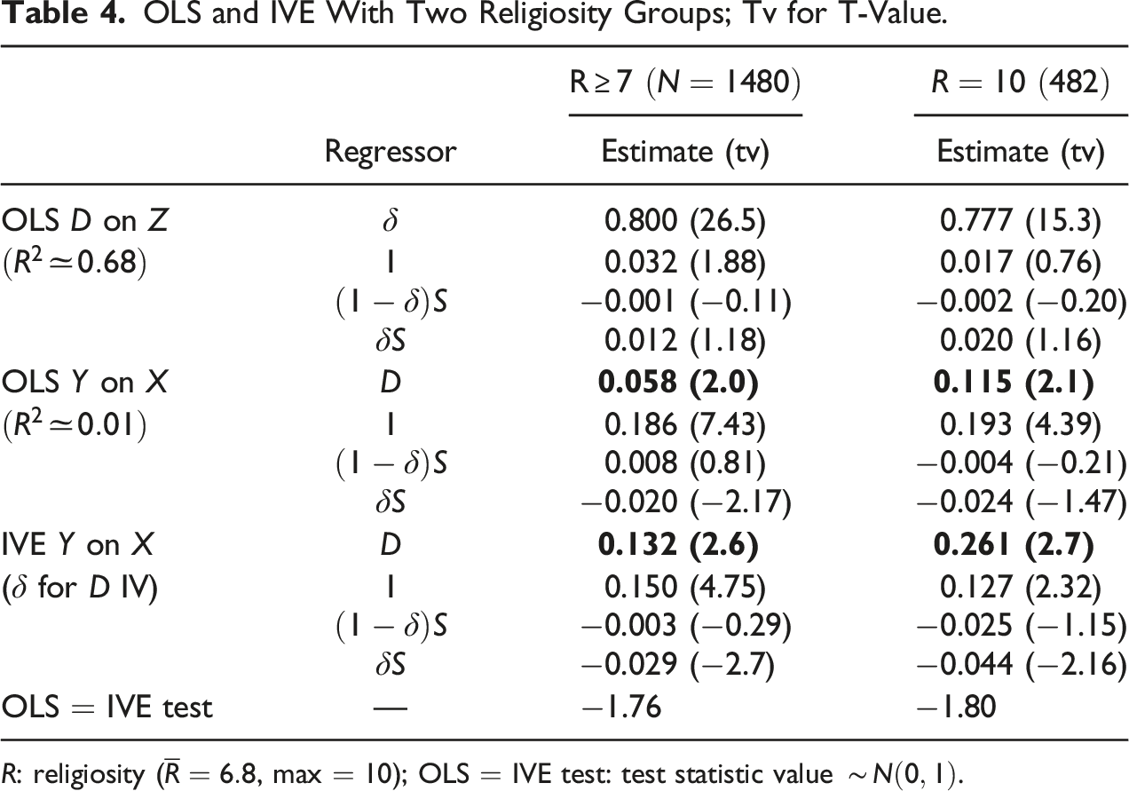
Table 4 presents the OLS of

D

Z

, the OLS of

Y

X

, and the IVE of

Y

X

. The rows for

D

are in a different font to make it easy to compare them. The OLS of

D

Z

shows that

δ

is highly influential for

D

because most eligible people for the program received the subsidy.

Table 4.

OLS and IVE With Two Religiosity Groups; Tv for T-Value.

	Regressor	$R \geq 7$ $(N = 1480)$	$R = 10$ $(482)$
	Regressor	Estimate (tv)	Estimate (tv)
OLS $D$ on $Z$	$δ$	0.800 (26.5)	0.777 (15.3)
$(R^{2} ≃ 0.68)$	$1$	0.032 (1.88)	0.017 (0.76)
	$(1 - δ) S$	−0.001 (−0.11)	−0.002 (−0.20)
	$δ S$	0.012 (1.18)	0.020 (1.16)
OLS $Y$ on $X$	$D$	0.058 (2.0)	0.115 (2.1)
$(R^{2} ≃ 0.01)$	$1$	0.186 (7.43)	0.193 (4.39)
	$(1 - δ) S$	0.008 (0.81)	−0.004 (−0.21)
	$δ S$	−0.020 (−2.17)	−0.024 (−1.47)
IVE $Y$ on $X$	$D$	0.132 (2.6)	0.261 (2.7)
( $δ$ for $D$ IV)	$1$	0.150 (4.75)	0.127 (2.32)
	$(1 - δ) S$	−0.003 (−0.29)	−0.025 (−1.15)
	$δ S$	−0.029 (−2.7)	−0.044 (−2.16)
OLS $=$ IVE test	—	−1.76	−1.80

$R$ : religiosity ( $\bar{R} = 6.8$ , max $= 10$ ); OLS $=$ IVE test: test statistic value $\sim N (0,1)$ .

In Table 4, the treatment effect of $D$ on $Y$ is increasing as the religiosity $R$ goes up, and the OLS under-estimates the treatment effect severely because the OLS effect is only $0.058 \sim 0.115$ , whereas the IVE effect is $0.132 \sim 0.261$ . We test for the difference in the last row, where an asymptotically standard normal test statistic value is presented for the null hypothesis that the effect parameters are the same in the OLS and IVE: the test statistic values are on the “borderline” of rejecting the null hypothesis. There are reasons to make the receipt of the subsidy $D$ endogenous; for example, for an eligible (i.e., $δ = 1$ ) individual to take up the subsidy, he/she might have to overcome the “stigma” of receiving the subsidy, and this psychological burden may be related to $Y$ .

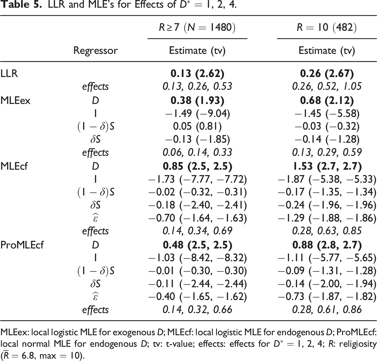
In Table 5, “ProMLEcf” is the same as MLEcf except that

E (Y | D, S, ε) = Φ (W^{'} β_{w})

is used instead of (14). To ease reading Table 5, the mean effects for

D^{*} = 1, 2, 4

are in italics, and the estimates for

β_{d}

and their t-values are in bold font. When two t-values appear in many entries for MLEcf and ProMLEcf, the first one ignores the error

\hat{ε} - ε

, while the second takes it into account. The difference between the two t-values is always very small, and thus, it seems safe to use the simpler t-value ignoring

\hat{ε} - ε

. As well known, logit estimates and probit estimates are almost the same, once the probit estimates are multiplied by

1.8

because

S D (logistic distribution) ≃ 1.8

. This is also the case in Table 5, and the effect estimates based on (19)(i) and

Φ (β_{d} d + β_{0}) - Φ (β_{0})

are nearly identical. Hence, we will no longer mention ProMLEcf.

Table 5.

LLR and MLE’s for Effects of $D^{*} = 1, 2, 4$ .

	Regressor	$R \geq 7$ $(N = 1480)$	$R = 10$ $(482)$
	Regressor	Estimate (tv)	Estimate (tv)
LLR		0.13 (2.62)	0.26 (2.67)
LLR	effects	0.13, 0.26, 0.53	0.26, 0.52, 1.05
MLEex	$D$	0.38 (1.93)	0.68 (2.12)
	$1$	−1.49 (−9.04)	−1.45 (−5.58)
	$(1 - δ) S$	0.05 (0.81)	−0.03 (−0.32)
	$δ S$	−0.13 (−1.85)	−0.14 (−1.28)
	effects	0.06, 0.14, 0.33	0.13, 0.29, 0.59
MLEcf	$D$	0.85 (2.5, 2.5)	1.53 (2.7, 2.7)
	$1$	−1.73 (−7.77, −7.72)	−1.87 (−5.38, −5.33)
	$(1 - δ) S$	−0.02 (−0.32, −0.31)	−0.17 (−1.35, −1.34)
	$δ S$	−0.18 (−2.40, −2.41)	−0.24 (−1.96, −1.96)
	$\hat{ε}$	−0.70 (−1.64, −1.63)	−1.29 (−1.88, −1.86)
	effects	0.14, 0.34, 0.69	0.28, 0.63, 0.85
ProMLEcf	$D$	0.48 (2.5, 2.5)	0.88 (2.8, 2.7)
	$1$	−1.03 (−8.42, −8.32)	−1.11 (−5.77, −5.65)
	$(1 - δ) S$	−0.01 (−0.30, −0.30)	−0.09 (−1.31, −1.28)
	$δ S$	−0.11 (−2.44, −2.44)	−0.14 (−2.00, −1.94)
	$\hat{ε}$	−0.40 (−1.65, −1.62)	−0.73 (−1.87, −1.82)
	effects	0.14, 0.32, 0.66	0.28, 0.61, 0.86

MLEex: local logistic MLE for exogenous $D$ ; MLEcf: local logistic MLE for endogenous $D$ ; ProMLEcf: local normal MLE for endogenous $D$ ; tv: t-value; effects: effects for $D^{*} = 1, 2, 4$ ; $R$ : religiosity ( $\bar{R} = 6.8$ , max $= 10$ ).

The slope of $D$ estimated by MLEex and MLEcf is the structural form parameter $β_{d}$ residing in the logistic distribution function, and its estimates are much greater than the LLR estimate. But looking at the mean effect $D = 1$ versus $D = 0$ , the mean effects are almost the same except for MLEex: $0.13 \sim 0.14$ for $R \geq 7$ , and $0.26 \sim 0.28$ for $R = 10$ . This degree of similarity is remarkable. The mean effects, however, diverge as we look at $D^{*} = 2, 4$ versus $D^{*} = 0$ . The mean effects based on the logit structural form parameter respect the bound $[- 1, 1]$ .

According to Table 4, the effect of $D = 1$ by IVE is $0.13 \sim 0.26$ depending on $R$ , and the same effects can be seen in the LLR row of Table 5. The “effects” row just below the LLR row shows the effects of $D^{*} = 1$ for $$ 35$ subsidy, $D^{*} = 2$ for $$ 70$ , and $D^{*} = 4$ for $$ 140$ using the linear extrapolation as in (3). Although the linear extrapolation works fine when the effect magnitude is small, it goes over the bound $[- 1, 1]$ when $D^{*}$ becomes large in the most religious group with $R = 10$ , which demonstrates our main point.

Is $D$ endogenous? The t-values of $\hat{ε}$ in Table 5 give borderline test statistic values as the last row of Table 4 does. Despite much difference in the linear models for Table 4 and non-linear ones for Table 5, seeing this level of coherence is reassuring. Despite the border line test statistic values, we would take the effect estimates allowing the $D$ endogeneity for two reasons. First, the conventional test level $(5 %)$ is too conservative, intended to make it difficult to reject the null hypothesis lest the rejection results in a much greater harm than otherwise, which is, however, unwarranted in our test; that is, raising the test level slightly results in rejecting the $D$ exogeneity. Second, for $D = 1$ , the three estimators (LLR, MLEcf, and ProMLEcf) give the almost identical estimates $(0.13 \sim 0.14)$ in unison: after all, the goal is estimating treatment effects at the possible presence of $D$ endogeneity, which is allowed by the three estimators without necessarily concluding the $D$ endogeneity or exogeneity.

Conclusions

Regression discontinuity (RD) estimators are often applied to binary response $Y = 0, 1$ with binary treatment $D = 0, 1$ without any modification. As when linear models are applied to binary responses, this practice typically does not pose problems. However, a problem occurs when we want to extrapolate the treatment from $D = 1$ to a number higher than $1$ , because the estimated effect for the new treatment may go out of the bound $[- 1, 1]$ which should hold for changes in $P (Y = 1 | \cdot)$ . A solution to this problem is estimating the structural form effect parameter for $D$ that appears inside a proper regression function for $Y$ , that is, a probability distribution function. We explored this line of approach in this paper, using the logistic distribution.

Specifically, for sharp RD, we proposed “local logistic MLE,” which is nothing but the usual logistic MLE using a local sample around the RD cutoff point $c$ . For fuzzy RD, we proposed a two-stage procedure, where the first stage is the ordinary least squares estimator (OLS) of $D$ on some regressors including the dummy for the RD running variable $S$ crossing $c$ , and the second stage is the local logistic MLE using the first-stage OLS residual as an extra regressor to control for the source of the possible endogeneity of $D$ .

The popular local linear regression (LLR) for RD amounts to applying instrumental variable estimator to a local linear model, which is the same as applying OLS to the $Y$ equation while using the $D$ -equation OLS residual as an extra regressor. In essence, our approach allowing endogenous treatment does the same, but with the logistic distribution function to respect the bound $[0, 1]$ for $P (Y = 1 | \cdot)$ . Through a simulation study, we showed that our local logistic MLE dominates LLR in the sense that both give almost the same estimates for the effect of $D = 1$ relative to $D = 0$ , but only our approach gives valid estimates for larger values of $D$ such as $2, 4$ .

We applied our proposed methods to a data set where $D$ is an income subsidy program and $Y$ is being Evangelical. The empirical analysis illustrated the aforementioned pitfall of LLR: when the income subsidy amount quadrupled, the effect on $P (Y = 1 | \cdot)$ turned out to be higher than one. In contrast, our approach of estimating structural form parameters gave effects respecting the bound $[- 1, 1]$ . Other than this, the effect estimates for the original treatment $D = 1$ in LLR and our approach were remarkably close. We were thus able to maintain the popular LLR for $D = 1$ , while overcoming the LLR bound problem in extrapolating the treatment dose, which was the very motivation for this paper.

Footnotes

Acknowledgments

The authors are grateful to the Editor and two anonymous reviewers for their helpful comments. This paper was originally circulated as a single-authored paper of Myoung-jae Lee, and Goeun Lee came on board contributing extra seven pages in the final version to tighten the theoretical part of the paper.

Declaration of Conflicting Interests

The author(s) declared no potential conflicts of interest with respect to the research, authorship, and/or publication of this article.

Funding

The author(s) disclosed receipt of the following financial support for the research, authorship, and/or publication of this article: The research of Myoung-jae Lee has been supported by a Korea University research grant.

ORCID iD

Goeun Lee

Appendix A: More Discussion on Choosing Bandwidth with Cross-Validation (CV)

For RD, Ludwig and Miller (2007) considered “one-sided CV” minimizing

Ω_{N}^{ω} (h) \equiv \sum_{i} ω_{i}^{h} {\{Y_{i} - {\hat{E}}_{- i} (Y {| S}_{i}, h)\}}^{2} / \sum_{i} ω_{i}^{h}

where

{\hat{E}}_{- i} (Y {| S}_{i}, h)

is defined as, depending on

S_{i} ≶ 0,

\frac{\sum_{j \neq i} K (\frac{(S_{j} - S_{i})}{h}) 1 [S_{j} < S_{i} < 0] Y_{j}}{\sum_{j \neq i} K (\frac{(S_{j} - S_{i})}{h}) 1 [S_{j} < S_{i} < 0]} or \frac{\sum_{j \neq i} K (\frac{(S_{j} - S_{i})}{h}) 1 [0 < S_{i} < S_{j}] Y_{j}}{\sum_{j \neq i} K (\frac{(S_{j} - S_{i})}{h}) 1 [0 < S_{i} < S_{j}]},

and

ω_{i}^{h} = 1

for

S_{i}

with at least some observations on its right when

S_{i} > 0

, and on its left when

S_{i} < 0

The idea for ${\hat{E}}_{- i} (Y {| S}_{i}, h)$ is simple: if $S_{i} < 0$ , then only the left observations with $S_{j} < S_{i}$ are used; if $0 < S_{i}$ , only the right observations with $S_{i} < S_{j}$ are used. However, $Ω_{N}^{ω} (h)$ tends to give too large a bandwidth that makes most $ω_{i}^{h}$ ’s zero and predicts the few remaining $Y_{i}$ ’s well to make $Ω_{N}^{ω} (h)$ small, which happened in Ludwig and Miller (2007), and Choi and Lee (2018a) as well for a two-dimensional $S$ . Although ${\tilde{E}}_{- i} (Y {| S}_{i}, h)$ is inconsistent for $E (Y | S = S_{i})$ when $S_{i}$ is near zero and $E (Y | S)$ has a break at $0$ , since the goal is finding a reasonable value of $h$ , not necessarily predicting $Y$ well, we recommend the conventional CV in the main text as Choi and Lee (2018a) did. In the empirical analysis of Choi and Lee (2018a), the conventional CV gave $h$ values similar to $h_{r u l e}$ .

Appendix B: Indirect Ratio-Based Approach for FRD Extrapolation

Here we provide the details on the indirect approach for FRD similar to (2), drawing partly on Choi and Lee (2018b). The discussion here reveals what kind of conditions are needed for the indirect approach, and why it fails in binary treatment extrapolation for binary outcome.

As in the main text, our non-binary treatment $D^{*}$ is

SRD: $D^{*} = d \times δ$ ( $= 0$ , $d$ , depending on $δ = 0, 1$ );

FRD: $D^{*} = d \times {(1 - δ) D^{0} + δ D^{1}}$ ( $= d \times D^{0}$ , $d \times D^{1}$ , depending on $δ = 0, 1$ ).

With the potential response $Y^{d}$ for $D^{*} = d$ , the “realized” response is

\begin{aligned} Y = Y^{0} + (Y^{d} - Y^{0}) D^{*} / d = Y^{0} + (Y^{d} - Y^{0}) D \\ = Y^{0} when D^{*} = 0 and Y^{d} when D^{*} = d \Leftrightarrow D = 1 . \end{aligned}

Note that we use the term “realized” instead of “observed” because

Y^{d}

is never observed for the counterfactual extrapolated treatment

D^{*} = d > 1

It is important to bear in mind that, even when $D^{*} = d > 1$ , $(D^{0}, D^{1})$ still take only on $0, 1$ ; it is just that the treatment dose is $d$ , not $1$ , when extrapolatedly treated. This setup is necessary for compliers to be defined still as $(D^{1} = 1, D^{0} = 0)$ regardless of $d$ . Maintaining this complier definition that does not change when $D^{*} = d > 1$ allowed is unavoidable, because only $D = 0, 1$ are realized. If the complier group changes as $d$ does, then we cannot identify the treatment effect on compliers for $D^{*} = d > 1$ . To simplify notation, define

Δ Y^{d} \equiv Y^{d} - Y^{0} .

Recall

ε \equiv D - E (D | S)

, which implies that

ε = 0

is equivalent to

D = δ

(i.e., complier). Putting all of requisite assumptions for the indirect approach in advance, they are: (22)

\begin{array}{l} (i) : E (Y^{0} | 0^{+}) = E (Y^{0} | 0^{-}); \\ (i i) : E (Δ Y^{d} \cdot D^{0} | 0^{+}) = E (Δ Y^{d} \cdot D^{0} | 0^{-}); \\ (i i i) : E (D^{0} | 0^{+}) = E (D^{0} | 0^{-}); \\ (i v) : D^{0} \leq D^{1} on S \in (0, ν) for an arbitrarily small constant ν > 0; \\ (v) : lim_{s ↓ 0} E (Δ Y^{d} | D^{1} - D^{0} = 1, S = s) and lim_{s ↓ 0} P (D^{1} - D^{0} = 1 | S = s) exist; \\ (v i) : E (D^{1} | 0^{+}) \neq E (D^{0} | 0^{-}) . \end{array}

Among these assumptions, (i)-(iii) are the continuity of

E (Y^{0} | S = s)

E (Δ Y^{d} \cdot D^{0} | S = s)

and

E (D^{0} | S = s)

s = 0

, respectively; (i) was assumed in Hahn et al. (2001), and (ii) and (iii) are weaker than the assumption

(Δ Y^{1}, D^{0}, D^{1}) ∐ S

S \in (- ν, ν)

in Hahn et al. (2001) when

d = 1

. The “monotonicity condition” (iv) is weaker than “

D^{0} \leq D^{1}

S \in (- ν, ν)

” in Hahn et al. (2001), and the condition rules out

D^{1} - D^{0} = - 1

so that

D^{1} - D^{0}

takes only on

0, 1

. (22)(v) is hardly a restriction, because it requires only the existence of the right limits at

s = 0

, not the continuities at

s = 0

. Finally, (22)(vi) is the usual break assumption of

E (D | S = s)

in FRD at

s = 0

, so that the treatment break is not zero at

s = 0

, even if the break magnitude is not one as in SRD.

Take $E (\cdot | 0^{+})$ and $E (\cdot | 0^{-})$ on the realized response $Y = Y^{0} + (Y^{d} - Y^{0}) D$ to get (23)

\begin{array}{l} E (Y | 0^{+}) = E (Y^{0} | 0^{+}) + E (Δ Y^{d} \cdot D | 0^{+}), \\ E (Y | 0^{-}) = E (Y^{0} | 0^{-}) + E (Δ Y^{d} \cdot D | 0^{-}) . \end{array}

Replace the two

D

’s in (23) with

D^{0}

and

D^{1}

, respectively, because

D = D^{1}

given

S > 0

, and

D = D^{0}

given

S < 0 :

(24)

\begin{array}{l} E (Y | 0^{+}) = E (Y^{0} | 0^{+}) + E (Δ Y^{d} \cdot D^{1} | 0^{+}), \\ E (Y | 0^{-}) = E (Y^{0} | 0^{-}) + E (Δ Y^{d} \cdot D^{0} | 0^{-}) . \end{array}

Take the difference of the two equations in (24) to remove

E (Y^{0} | 0^{+})

and

E (Y^{0} | 0^{-})

due to (22)(i). This gives (25)

E (Y | 0^{+}) - E (Y | 0^{-}) = E (Δ Y^{d} \cdot D^{1} | 0^{+}) - E (Δ Y^{d} \cdot D^{0} | 0^{-}) .

Invoke (22)(ii) to replace

E (Δ Y^{d} \cdot D^{0} | 0^{-})

with

E (Δ Y^{d} \cdot D^{0} | 0^{+})

, so that (25) can be written succinctly as (26)

\begin{array}{l} E (Y | 0^{+}) - E (Y | 0^{-}) = E \{Δ Y^{d} \cdot (D^{1} - D^{0}) | 0^{+}\} \\ \equiv lim_{s ↓ 0} E \{Δ Y^{d} \cdot (D^{1} - D^{0}) | S = s\} (definition of E \{Δ Y^{d} \cdot (D^{1} - D^{0}) | 0^{+}\}) \\ = lim_{s ↓ 0} E (Δ Y^{d} | D^{1} - D^{0} = 1, S = s) P (D^{1} - D^{0} = 1 | S = s) (due to (22) (iv)) \\ = E (Δ Y^{d} | D^{1} - D^{0} = 1, 0^{+}) P (D^{1} - D^{0} = 1 | 0^{+}) (due to (22) (v)) . \end{array}

Invoke (22)(iii) to see

E (D | 0^{+}) - E (D | 0^{-}) = E (D^{1} | 0^{+}) - E (D^{0} | 0^{-}) = E (D^{1} - D^{0} | 0^{+})

= P (D^{1} - D^{0} = 1 | 0^{+})

(due to the monotonicity (22)(iv)).Substituting this into

P (D^{1} - D^{0} = 1 | 0^{+})

in (26), the first and last terms of (26) render

E (Y | 0^{+}) - E (Y | 0^{-}) = E (Δ Y^{d} | D^{1} - D^{0} = 1, 0^{+}) \{E (D | 0^{+}) - E (D | 0^{-})\} .

Under the

D

-break assumption in (22)(vi), this can be rewritten as (27)

E (Y^{d} - Y^{0} | D^{1} > D^{0}, 0^{+}) = \frac{E (Y | 0^{+}) - E (Y | 0^{-})}{E (D | 0^{+}) - E (D | 0^{-})} = \frac{E (Y^{d} | 0^{+}) - E (Y^{0} | 0^{-})}{E (D^{1} | 0^{+}) - E (D^{0} | 0^{-})} .

The ratio in (2) can be defined as

β_{1}

because it is the effect of

D

changing from

0

1

. Analogously, we can define the ratio in (27) as

β_{d}

because it is the effect of

D^{*}

changing potentially from

0

d

(with

D

changing from

0

1

): (28)

β_{d} \equiv \frac{E (Y | 0^{+}) - E (Y | 0^{-})}{E (D | 0^{+}) - E (D | 0^{-})} = \frac{E (Y^{d} | 0^{+}) - E (Y^{0} | 0^{-})}{E (D^{1} | 0^{+}) - E (D^{0} | 0^{-})} .

The point is that the assumptions in (22) do not imply

E (Y^{d} | 0^{+}) - E (Y^{0} | 0^{-}) = d {E (Y^{1} | 0^{+}) - E (Y^{0} | 0^{-})}

. That is, in the indirect approach, there is no guarantee for (29)

β_{d} \equiv \frac{E (Y^{d} | 0^{+}) - E (Y^{0} | 0^{-})}{E (D^{1} | 0^{+}) - E (D^{0} | 0^{-})} = d \times \frac{E (Y^{1} | 0^{+}) - E (Y^{0} | 0^{-})}{E (D^{1} | 0^{+}) - E (D^{0} | 0^{-})} \equiv d \times β_{1},

although this is what is needed for the linear extrapolation (3).

(29) reveals that the indirect approach based on localization around $S = 0$ is not well suited for extrapolation. Instead, our direct approach using the control function $ε \equiv D - E (D | S)$ with a proper distribution function (such as the logistic distribution function) can be used to rein in the misleading linear growth as $d$ goes up in the linear extrapolation. Of course, the price to pay is specifying the parametric distribution function, but the price is almost zero, as long as the direct approach gives almost the same results as the indirect approach gives for $D = 0, 1$ . This was amply demonstrated in our simulation and empirical studies.

Appendix C: Proof for Equivalence E ( D | S ) = α δ δ + m D ( S ) ⇔ α δ ≡ E ( D | 0 + ) − E ( D | 0 − )

First, take $E (\cdot | 0^{+})$ and $E (\cdot | 0^{-})$ on $E (D | S) = α_{δ} δ + m_{D} (S)$ to get, as $m_{D} (0^{+}) = m_{D} (0^{-}),$

E (D | 0^{+}) = α_{δ} + m_{D} (0^{+}), E (D | 0^{-}) = m_{D} (0^{-}) \Rightarrow α_{δ} = E (D | 0^{+}) - E (D | 0^{-}) .

Hence, “

E (D | S) = α_{δ} δ + m_{D} (S)

” implies “

α_{δ} = E (D | 0^{+}) - E (D | 0^{-})

”.

Second, for the reverse, define $m_{D} (S) \equiv E (D | S) - α_{δ} δ$ using the local mean difference $α_{δ}$ , and take $E (\cdot | 0^{+})$ and $E (\cdot | 0^{-})$ on $m_{D} (S) :$

\begin{array}{l} m_{D} (0^{+}) \equiv E (D | 0^{+}) - α_{δ}, m_{D} (0^{-}) \equiv E (D | 0^{-}) \\ \Rightarrow m_{D} (0^{+}) - m_{D} (0^{-}) = E (D | 0^{+}) - E (D | 0^{-}) - α_{δ} . \end{array}

“

α_{δ} \equiv E (D | 0^{+}) - E (D | 0^{-})

” implies

m_{D} (0^{+}) - m_{D} (0^{-}) = 0

, which is the continuity of

m_{D} (S)

0

. Hence,

E (D | S) = α_{δ} δ + m_{D} (S)

with

m_{D} (S)

continuous at

0

follows from the definition

m_{D} (S) \equiv E (D | S) - α_{δ} δ

Appendix D: Asymptotic Distribution for Local Logistic MLE with Control Function

Let $Λ (\cdot)$ and $λ (\cdot)$ be the logistic distribution and density functions, respectively:

Λ (W^{'} β_{w}) \equiv \frac{\exp (W^{'} β_{w})}{1 + \exp (W^{'} β_{w})} and  λ (W^{'} β_{w}) = \frac{\exp (W^{'} β_{w})}{{\{1 + \exp (W^{'} β_{w})\}}^{2}} .

The score function for the logistic MLE is then

T \equiv \frac{\{Y - Λ (W^{'} β_{w})\} \cdot λ (W^{'} β_{w})}{Λ (W^{'} β_{w}) \{1 - Λ (W^{'} β_{w})\}} W .

Let

\hat{T}

denote

T

with

W

and

β_{w}

replaced by

\hat{W}

and

{\hat{β}}_{w}

It holds that

{\hat{β}}_{w} - β_{w} = - {(\sum_{i} Q_{i} {\hat{T}}_{i} {\hat{T}}_{i}^{'})}^{- 1} \cdot \sum_{i} Q_{i} {\hat{T}}_{i} + o_{p} (1 / \sqrt{N h}) .

Although tedious, it can be shown that the presence of

\hat{ε}

\hat{W}

matters only for

Y - Λ (W^{'} β_{w})

, which gives (

o_{p} (1 / \sqrt{N h})

terms omitted)

\begin{array}{l} {\hat{β}}_{w} - β_{w} = - (\sum_{i} Q_{i} T_{i} T_{i}^{'})^{- 1} \sum_{i} Q_{i} \frac{\{Y - Λ ({\hat{W}}_{i}^{'} β_{w})\} \cdot λ (W_{i}^{'} β_{w})}{Λ (W_{i}^{'} β_{w}) \{1 - Λ (W_{i}^{'} β_{w})\}} W_{i} \\ = - (\sum_{i} Q_{i} T_{i} T_{i}^{'})^{- 1} \sum_{i} [Q_{i} T_{i} - Q_{i} \frac{λ {(W_{i}^{'} β_{w})}^{2}}{Λ (W_{i}^{'} β_{w}) \{1 - Λ (W_{i}^{'} β_{w})\}} W_{i} β_{w}^{'} ({\hat{W}}_{i} - W_{i})] \end{array}

using the linear approximation

Λ ({\hat{W}}_{i}^{'} β_{w}) ≃ Λ (W_{i}^{'} β_{w}) + λ (W_{i}^{'} β_{w}) β_{w}^{'} ({\hat{W}}_{i} - W_{i})

Observe

\hat{W} - W = [\begin{matrix} D \\ 1 \\ (1 - δ) S \\ δ S \\ D - Z^{'} \hat{α} \end{matrix}] - [\begin{matrix} D \\ 1 \\ (1 - δ) S \\ δ S \\ ε \end{matrix}] ≃ A \cdot Z^{'} (\hat{α} - α) where A \equiv [\begin{matrix} 0 \\ 0 \\ 0 \\ 0 \\ - 1 \end{matrix}] .

Because

\hat{α} - α = {(\sum_{i} Q_{i} Z_{i} Z_{i}^{'})}^{- 1} \sum_{i} Q_{i} Z_{i} ε_{i} + o_{p} (1 / \sqrt{N h}),

we have, omitting

o_{p} (1 / \sqrt{N h})

terms again,

\begin{array}{l} {\hat{β}}_{w} - β_{w} = - {(\sum_{i} Q_{i} T_{i} T_{i}^{'})}^{- 1} \cdot \sum_{i} [Q_{i} T_{i} \\ - Q_{i} \frac{λ {(W_{i}^{'} β_{w})}^{2} β_{w}^{'} A}{Λ (W_{i}^{'} β_{w}) \{1 - Λ (W_{i}^{'} β_{w})\}} W_{i} Z_{i}^{'} \cdot {(\sum_{i} Q_{i} Z_{i} Z_{i}^{'})}^{- 1} \sum_{i} Q_{i} Z_{i} ε_{i}] \end{array}

Since

β_{w}^{'} A = - β_{ε}

, this can be written as

\begin{array}{l} {\hat{β}}_{w} - β_{w} = - (\sum_{i} Q_{i} T_{i} T_{i}^{'})^{- 1} \cdot \sum_{i} [Q_{i} T_{i} \\ + β_{ε} Q_{i} \frac{λ {(W_{i}^{'} β_{w})}^{2}}{Λ (W_{i}^{'} β_{w}) \{1 - Λ (W_{i}^{'} β_{w})\}} W_{i} Z_{i}^{'} \cdot (\sum_{i} Q_{i} Z_{i} Z_{i}^{'})^{- 1} \sum_{i} Q_{i} Z_{i} ε_{i}]. \end{array}

Define

\begin{array}{l} H \equiv \sum_{i} Q_{i} {[\frac{\{Y_{i} - Λ (W_{i}^{'} β_{w})\} \cdot λ (W_{i}^{'} β_{w})}{Λ (W_{i}^{'} β_{w}) \{1 - Λ (W_{i}^{'} β_{w})\}}]}^{2} W_{i} W_{i}^{'} and \\ C_{i} \equiv \frac{λ {(W_{i}^{'} β_{w})}^{2}}{Λ (W_{i}^{'} β_{w}) \{1 - Λ (W_{i}^{'} β_{w})\}} W_{i} Z_{i}^{'} \cdot (\sum_{i} Q_{i} Z_{i} Z_{i}^{'})^{- 1}; \end{array}

also define

\hat{H}

and

{\hat{C}}_{i}

H

and

C_{i}

with

(W_{i}, β_{w})

replaced by

({\hat{W}}_{i}, {\hat{β}}_{w})

. Now, rewrite

{\hat{β}}_{w} - β_{w}

{\hat{β}}_{w} - β_{w} = - H^{- 1} \sum_{i} Q_{i} [T_{i} + β_{ε} \frac{λ {(W_{i}^{'} β_{w})}^{2}}{Λ (W_{i}^{'} β_{w}) \{1 - Λ (W_{i}^{'} β_{w})\}} W_{i} Z_{i}^{'} (\sum_{i} Q_{i} Z_{i} Z_{i}^{'})^{- 1} \cdot Z_{i} ε_{i}] .

This shows that the asymptotic variance of

{\hat{β}}_{w}

can be estimated with

{\hat{H}}^{- 1} \sum_{i} Q_{i} {\hat{ξ}}_{i} {\hat{ξ}}_{i}' {\hat{H}}^{- 1} where {\hat{ξ}}_{i} \equiv \frac{{Y - Λ ({\hat{W}}_{i}' {\hat{β}}_{w})} λ ({\hat{W}}_{i}' {\hat{β}}_{w})}{Λ ({\hat{W}}_{i}' {\hat{β}}_{w}) {1 - Λ ({\hat{W}}_{i}' {\hat{β}}_{w})}} {\hat{W}}_{i} + {\hat{β}}_{ε} {\hat{C}}_{i} Z_{i} {\hat{ε}}_{i} .

The second term of

\hat{ξ}

is the “correction term” accounting for

\hat{ε} - ε

, which drops out under the null hypothesis

β_{ε} = 0

; that is, under the null hypothesis of

D

exogeneity,

\hat{ε} - ε

can be ignored. This way of accounting for the first-stage error can be found in Lee (2010), among others.

References

Angrist

Rokkanen

(2015). Wanna get away? Regression discontinuity estimation of exam school effects away from the cutoff. Journal of the American Statistical Association, 110(512), 1331–1344. https://doi.org/10.1080/01621459.2015.1012259

Angrist

J. D.

Imbens

G. W.

Rubin

D. B.

(1996). Identification of causal effects using instrumental variables. Journal of the American Statistical Association, 91(434), 444–455. https://doi.org/10.1080/01621459.1996.10476902

Berk

de Leeuw

(1999). An evaluation of California’s inmate classification system using a generalized regression discontinuity design. Journal of the American Statistical Association, 94(448), 1045–1052. https://doi.org/10.1080/01621459.1999.10473857

Berk

Rauma

(1983). Capitalizing on nonrandom assignment to treatments: A regression-discontinuity evaluation of a crime control program. Journal of the American Statistical Association, 78(381), 21–27. https://doi.org/10.1080/01621459.1983.10477917

Buser

(2015). The effect of income on religiousness. American Economic Journal: Applied Economics, 7(3), 178–195. https://doi.org/10.1257/app.20140162

Calonico

Cattaneo

Titiunik

(2014). Robust nonparametric confidence intervals for regression-discontinuity designs. Econometrica, 82(6), 2295–2326. https://doi.org/10.3982/ecta11757

Card

Lee

Pei

Weber

(2017). Regression kink design: Theory and practice, advances in econometrics 38. In Cattaneo

M. D.

Escanciano

J. C.

(Eds.). Emerald Publishing Limited.

Cattaneo

M. D.

Escanciano

J. C.

(2017). Introduction, advances in econometrics 38 (entitled ‘Regression discontinuity designs: Theory and applications’). In Cattaneo

M. D.

Escanciano

J. C.

(Eds.). Emerald Publishing.

Cattaneo

M. D.

Idrobo

Titiunik

(2019). A practical introduction to regression discontinuity designs. Cambridge University Press. https://doi.org/10.1017/9781108684606

10.

Choi

J. Y.

Lee

M. J.

(2017). Regression discontinuity: Review with extensions. Statistical Papers, 58(4), 1217–1246. https://doi.org/10.1007/s00362-016-0745-z

11.

Choi

J. Y.

Lee

M. J.

(2018a). Regression discontinuity with multiple running variables allowing partial effects. Political Analysis, 26(3), 258–274. https://doi.org/10.1017/pan.2018.13

12.

Choi

J. Y.

Lee

M. J.

(2018b). Relaxing conditions for local average treatment effect in fuzzy regression discontinuity. Economics Letters, 173, 47–50. https://doi.org/10.1016/j.econlet.2018.09.010

13.

Choi

J. Y.

Lee

M. J.

(2021). Basics and recent advances in regression discontinuity: Difference versus regression forms. Journal of Economic Theory and Econometrics, 32(3), 1–68. http://es.re.kr/eng/upload/jetem%2032-3-1.pdf

14.

Clarke

Windmeijer

(2012). Instrumental variable estimators for binary outcomes. Journal of the American Statistical Association, 107(500), 1638–1652. https://doi.org/10.1080/01621459.2012.734171

15.

Collins

A. M.

Klerman

J. A.

Briefel

Rowe

Gordon

A. R.

Logan

C. W.

Wolf

Bell

S. H.

(2018). A summer nutrition benefit pilot program and low-income children’s food security. Pediatrics, 141(4), Article e20171657. https://doi.org/10.1542/peds.2017-1657

16.

Dong

Lewbel

(2015). Identifying the effect of changing the policy threshold in regression discontinuity models. Review of Economics and Statistics, 97(5), 1081–1092. https://doi.org/10.1162/rest_a_00510

17.

Hahn

Todd

Van der Klaauw

(2001). Identification and estimation of treatment effects with a regression-discontinuity design. Econometrica, 69(1), 201–209. https://www.jstor.org/stable/2692190

18.

Imbens

G. W.

Angrist

(1994). Identification and estimation of local average treatment effects. Econometrica, 62(2), 467–475. https://doi.org/10.2307/2951620

19.

Imbens

G. W.

Kalyanaraman

(2012). Optimal bandwidth choice for the regression discontinuity estimator. Review of Economic Studies, 79(3), 933–959. https://doi.org/10.1093/restud/rdr043

20.

Imbens

G. W.

Lemieux

(2008). Regression discontinuity designs: A guide to practice. Journal of Econometrics, 142(2), 615–635. https://doi.org/10.1016/j.jeconom.2007.05.001

21.

Koch

Racine

(2016). Health care facility choice and user fee abolition: Regression discontinuity in a multinomial choice setting. Journal of the Royal Statistical Society (Series A), 179(4), 927–950. https://doi.org/10.1111/rssa.12161

22.

Lee

Lemieux

(2010). Regression discontinuity designs in economics. Journal of Economic Literature, 48(2), 281–355. https://doi.org/10.1257/jel.48.2.281

23.

Lee

M. J.

(2010). Micro-econometrics: Methods of moments and limited dependent variables. Springer.

24.

Lee

M. J.

(2012). Semiparametric estimators for limited dependent variable (LDV) models with endogenous regressors. Econometric Reviews, 31(2), 171–214. https://doi.org/10.1080/07474938.2011.607101

25.

Lee

M. J.

(2016). Matching, regression discontinuity, difference in differences, and beyond. Oxford University Press. https://doi.org/10.1093/acprof:oso/9780190258733.001.0001

26.

Ludwig

Miller

(2007). Does head start improve children’s life chances? Evidence from a regression discontinuity design. Quarterly Journal of Economics, 122(1), 159–208. https://doi.org/10.1162/qjec.122.1.159

27.

Sharma

McNeil

J. H.

(2009). To scale or not to scale: The principles of dose extrapolation. British Journal of Pharmacology, 157(6), 907–921. https://doi.org/10.1111/j.1476-5381.2009.00267.x

28.

K. L.

(2017). Regression discontinuity with categorical outcomes. Journal of Econometrics, 201(1), 1–18. https://doi.org/10.1016/j.jeconom.2017.07.004