Stasis and change in Holocene small mammal diversity during a period of aridification in southeastern Utah

Abstract

Biological conservation depends on understanding and disentangling the effects of decadal- to centennial-scale dynamics from the millennial-scale dynamics documented in the fossil record. The American Southwest is expected to become increasingly arid over the next few decades and will continue to experience large-scale human land use in various forms. A primary question is whether the ecological fluctuations recorded over the past few decades fall outside the range of variation expected in the absence of recent land use and management. I excavated and quantified mammal diversity change in two fossil-bearing alcoves, East Canyon Rims 2 and Rone Bailey Alcove, located in San Juan County, Utah. AMS radiocarbon dates on 33 bone samples from these sites span ~4.4–0.5 kyr and shed light on pre-industrial faunal dynamics in the region over the course of environmental change. Localities with comparable small mammal diversity have not been reported from this region previously, so these deposits provide novel insight into Holocene mammal diversity in southeastern Utah. Taxa recorded in these sites include leporids, sciurids, perognathines, arvicolines, Onychomys, Cynomys, Dipodomys, Peromyscus, Neotoma, and Thomomys. Using temporal cross-correlation, I tested for a relationship between regional temperature and species richness, evenness, relative abundance, and rank abundance. I also tested for changes in the overall taxon abundance distribution and visualized faunal relationships among time bins using non-metric multidimensional scaling of relative abundance data. None of the measures of diversity tested here were correlated with temperature change through time except for relative abundance of leporids. Overall, these results suggest that climatic fluctuations of the magnitude preserved in these deposits did not significantly alter the small mammal community, nor is there evidence that the presence, then exodus, of Native Americans from the region significantly affected small mammals.

Keywords

climate change Colorado Plateau conservation paleobiology diversity dynamics late Holocene small mammals

Introduction

The biodiversity of the Colorado Plateau (CP; southwestern United States) is threatened by both land use and climate change impacts. This region is 42% federally owned land (less than 14% is privately owned), and over 80% of that land is multi-use, including mining, grazing, energy development (fossil fuel and solar/wind), off-road vehicle travel, timber harvesting, hiking, fishing, hunting, and other activities (Ernst and Prior-Magee, 2008). Understanding ecological dynamics on these multi-use lands is crucial for preservation of the ecosystem services and intangible benefits they provide (Fu et al., 2015; Lawler et al., 2014; Nash, 1967). While much information is becoming available on ecological dynamics that operate over decadal and shorter time scales, we still know little about the over-lying long-term dynamics that are important in conservation efforts (Conservation Paleobiology Workshop, 2012; Dietl and Flessa, 2011; Dietl et al., 2015; Hadly and Barnosky, 2009; Kidwell, 2015; Rick and Lockwood, 2013; Swetnam et al., 1999; Willis and Birks, 2006). A primary question is whether the ecological fluctuations recorded over the past few decades fall outside the range of variation expected in the absence of recent land use and management. For example, to what extent do current relative abundances, distribution, and associations of species reflect recent adjustments of species due to anthropogenic pressures versus natural fluctuations that typify ecological dynamics that play out over millennia? Such questions can only be answered by tracing ecological dynamics through thousands of years, using the natural experiments preserved in the fossil record (Conservation Paleobiology Workshop, 2012; Hadly and Barnosky, 2009; Kidwell, 2015).

Biological conservation on the CP depends on understanding and disentangling the effects of decadal- to centennial-scale dynamics, such as grazing and other human impacts, from the millennial-scale dynamics documented in the fossil record. The American Southwest is expected to become increasingly arid over the next few decades: conditions analogous to previous multi-year droughts, including the Dust Bowl, are expected to become the norm (Seager et al., 2007). Under the A2 (highest) greenhouse gas emissions scenario, precipitation is estimated to decline by around 66% by 2090 and temperatures are expected to increase ~1.5–3°C by 2041–2070 and ~3–5°C by 2070–2090 (Garfin et al., 2014).

The effects of climate on biota can take many forms: mammals can shift their geographic range, population abundance, physiology, body size, phenology, and so on, or, if a species’ environmental tolerances are greater than the amount of environmental change expected, they may remain observably unaffected. Assessing community-level fluctuations is one way to synthesize these many responses and compare the whole mammal community from one time period to another. Detailed paleoecological records from Quaternary deposits have been remarkably useful in characterizing these millennial-scale ecological dynamics in other regions (Anderson, 1993; Anderson et al., 1999, 2000; Barnosky et al., 2004; Betancourt, 1984; Blois et al., 2010; Graham and Grimm, 1990; Grayson, 2011; Hadly, 1996). Past studies have detected a strong relationship between faunal composition and climate: in Samwell Cave (California), Blois et al. (2010) show a correlation between warming climate and declining species evenness and richness from ~17 to 1.5 kyr; Terry et al. (2011) found that cave deposits in the Great Basin record proportional increases in ‘southern affinity taxa’ when climate warmed and dried over the last ~7.5 kyr; and the Porcupine Cave (Colorado) pit sequence spanning 1 ma to ~600 kyr revealed little community change due to climate change except that small herbivores were less diverse during warm interglacial periods (Barnosky et al., 2004). However, while small mammals are important indicators of climate and environment, they do not always track vegetation (Graham and Grimm, 1990) or temperature and precipitation predictably. For example, Lamar Cave in Yellowstone records the presence of mesic-adapted taxa during time intervals that are considered warm/arid (Hadly, 1996). At Mescal Cave in the northern Mojave Desert, Stegner (2015) found that although both Neotoma cinerea and Marmota flaviventris are considered boreal-adapted, N. cinerea disappeared at the end of the Pleistocene while M. flaviventris was present at the site during several thousand years of Holocene warming and aridification.

Few Quaternary fossil records that sample the small mammal community of the CP have been studied to date (Carrasco et al., 2005; Emslie, 1986; FAUNMAP Working Group, 1994; Mead, 1981; Mead and Phillips, 1981; Tweet et al., 2012), particularly in southeastern Utah, where only a handful of Quaternary vertebrate localities have been published. Most of these contain fewer than five taxa – primarily large-bodied species – and few specimens (Carrasco et al., 2005; FAUNMAP Working Group, 1994, 1996). Archaeological and fossil plant records from the Quaternary CP, in contrast, have been more-extensively studied and provide an important context for new vertebrate fossil data presented here. Holocene rockshelter deposits are common across the CP (Mead et al., 2003; Tweet et al., 2012) and contain abundant small mammal remains that can be used to track the communities through long time spans. To this end, I excavated and quantified mammal diversity change in two fossil-bearing alcoves located in San Juan County, Utah. These localities, East Canyon Rims 2 (ECR2) and Rone Bailey Alcove (RBA), contribute to our understanding of natural variation in this system by providing faunal data for a period of recent climate change – a transition from generally cool-wet to warm-dry that occurred within the last 5 kyr. Accelerator Mass Spectrometry (AMS) radiocarbon dates on 33 bone samples from these sites span ~4400 cal. BP to present and shed light on pre-industrial faunal dynamics in the region over the course of environmental change, most notably aridification. Localities with comparable mammal diversity have not been reported from this region previously, so these sites provide novel insight into Holocene mammal diversity in southeastern Utah.

Study region

The CP is a physiogeographic province in North America centered on the Four Corners Region where Utah, Colorado, New Mexico, and Arizona meet. It is an arid region with high topographic relief – from ~900 to 4300 m – pocked with isolated laccolithic mountains and creased with deep canyons formed by the Colorado River and its tributaries (Barnes, 1993; Chronic, 1990). The CP is flanked to the west by the Great Basin, to the east by the Rocky Mountains, and to the south by the Sonoran and Chihuahuan Deserts. The western border is formed by a series of mountain ranges – the Uinta Mountains, Wasatch Range, and Fishlake and Aquarius Plateaus (Rowe, 2007) – while the Mogollon Rim in Arizona and the Rio Grande Rift Valley in New Mexico form the southwestern and southeastern borders, respectively (Foos, 1999).

Localities

RBA and ECR2 are large, horizontally shallow alcoves in the Slickrock Entrada Sandstone cliff face of Rone Bailey Mesa, Canyon Rims Recreation Area (BLM), San Juan County, Utah (Figure 1a–c). ECR2 is 1830 m (±5 m) in elevation, southeast-facing, and roughly ~50 m across, ~30 m high at the mouth, and ~20 m deep (Figure 1c). RBA is 1905 m (±5 m) in elevation and faces roughly southwest. RBA (~10 m high by ~3 m wide by ~5 m deep) is contained within a much larger alcove, and an apron of sediment roughly 10–15 m high extends from a maximum height at the midden, spilling southwest to the floor of the larger alcove (Figure 1b). Quaternary eolian sediments have accumulated in both ECR2 and RBA and buried bone and plant material collected by roosting raptors (as evidenced by raptor pellets on the surface of the sediments) and woodrats (genus Neotoma). Woodrats remain active at both sites today, and mammalian carnivores also may have played a role in bone accumulation in these middens.

Figure 1.

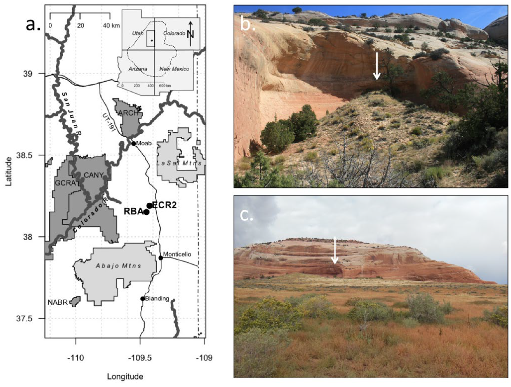
(a) Map of localities and geographic landmarks mentioned in the text; regional map is inset, the dashed line indicates the rough outline of the Colorado Plateau. (b) RBA from approximately west; arrow indicates location of woodrat midden deposit. (c) ECR2 from approximately south; arrow indicates location of woodrat midden deposit.

The vegetation surrounding these sites today is a patchy mixture of sagebrush-dominated areas, open perennial grassland, and pinyon–juniper woodland. Cooler and more mesic pockets harbor gambel oak (Quercus gambelii), barberry (Mahonia fremontii), squawbush (Rhus trilobata), Utah service berry (Amelanchier utahensis), and spruce (Picea englemannii). At ECR2, invasive Russian thistle (tumble weed, Salsola spp.) dominates the middle of the drainage where a primitive road passes through and forms dense patches up to approximately a meter high in places. Russian thistle is present near RBA as well, but it is sparser and does not produce the monotypic thickets seen near ECR2. The area around Rone Bailey Mesa has been grazed by cattle and horses for over a century (Lavender, 1964).

Climate and vegetation history of CP

Today, the CP marks the geographic transition between summer-wet (summer monsoon) to the south and summer-dry to the northwest (Anderson et al., 2000). Southeastern Utah currently experiences summer monsoons, but the monsoon boundary shifts through time in response to temperature, snow pack in the Rocky Mountains, location of the Jetstream, and other factors (Anderson et al., 2000). Because the CP has high topographic variability – deep canyons and high peaks – typical precipitation and temperature are spatially heterogeneous. However, most of the region receives between 4 and 12 inches of precipitation annually and experiences minimum January temperatures around −10°C to −4°C (13–25°F) and maximum July temperatures between roughly 29°C and 38°C (84–100°F) (30-year normals from 1981 to 2010) (PRISM Climate Group, 2015).

The CP was cooler and more mesic during the last glacial period of the Pleistocene, before ~14 kyr, at which time it was characterized by juniper woodland and sagebrush between ~600 and 1500 m; pinyon, limber pine, and Douglass fir between 1500 and 1800 m; Engelmann spruce/juniper forest around 2100 m; and spruce/pine forest above 2700 m (Anderson et al., 2000; Cole, 1990). Since the last glacial maximum, the dominant tree and shrub species – including Abies concolor (white fir), Artemisia spp. (sagebrush), Atriplex confertifolia (shadscale saltbush), Cercocarpus intricatus (mountain mahogany), Ephedra spp. (Mormon tea), Juniperus spp. (Juniper), Opuntia spp. (prickly pear), Picea spp. (Spruce), Pinus ponderosa (Ponderosa pine), Yucca angustissima (narrow-leaf yucca), and many others – have generally moved 700–900 m higher in elevation and 400–700 km up river (Cole, 1990). At the end of the Pleistocene, middens from the Abajos and Comb Ridge (respectively ~45 and ~85 km south of Rone Bailey Mesa) record a mixture of xeric- and mesic-adapted plants; the mesic components (e.g. subalpine conifers) of the flora disappeared from lower elevations, but modern dominant trees – pinyon (Pinus edulus and Pinus monophylla) and ponderosa (P. ponderosa) – did not appear at those elevations until the mid-Holocene (~7–3 kyr) (Betancourt, 1984; Coats et al., 2008). Pinyon has been expanding from south to north across the CP since the end of the glacial period (Coats et al., 2008).

With increasing elevation in this arid region, precipitation increases and temperature decreases on average (Betancourt, 1984). The fossil localities are between ~1830 and 1900 m in elevation, so the plant community likely progressed from pinyon, Douglas fir, and other conifers at the end of the Pleistocene, to juniper woodland and sagebrush with smaller pockets of ponderosa and spruce over the course of the Holocene, to an assemblage dominated by sagebrush and grasslands with large pockets of pinyon–juniper today. Preliminary analysis of pollen from RBA has identified spruce in the deepest excavation level, around 4400 cal. BP, and juniper throughout the deposit.

Climatically, the early Holocene was cooler than today, but more mesic than the late Glacial because the summer monsoon was strengthened (Weng and Jackson, 1999); this is also when the modern monsoon boundary was established (Betancourt, 1984). This cool mesic period gave way to an arid and warm mid-Holocene, from about 8.5 to 6 kyr (Reheis et al., 2005; Weng and Jackson, 1999). From ~6 to 3 kyr, cool-wet conditions returned (Reheis et al., 2005) and fossil plant evidence from the Abajos suggests higher effective moisture before 3 kyr (Betancourt, 1984). At the end of this period, around 3120 cal. BP, Maize agriculture arrived in this area as indicated by pollen in the Abajos records (Betancourt and Davis, 1984). Analysis of eolian and alluvial deposition in Canyonlands National Park suggests that from 2 kyr to the present drier conditions set in, as evidenced by greater mobility of dune sand (Reheis et al., 2005). In contrast, flood deposits from Utah and Arizona suggest drier periods from 3.6 to 2.2 kyr and 0.8 to 0.6 kyr, contrasted with peak flood magnitude and frequency from 1.1 to 0.9 kyr and again after 0.5 kyr (Ely, 1997). These peak floods are linked to increases in winter storms and dissipating tropical cyclones rather than summer precipitation or monsoon (Ely, 1997). Tree ring data record a mesic period from ~900 to 820 BP, followed by a series of at least six muti-decadal (>20 years) droughts – so-called megadroughts – that took place from ~1100 to 350 BP (Benson and Berry, 2009). The first of these megadroughts occurred between 1087 and 1066 BP (Benson and Berry, 2009). Human settlements in the northern San Juan Basin (southeastern Utah and southwestern Colorado) were largely abandoned by around 650 BP (Benson and Berry, 2009). Whether this exodus is attributable directly (e.g. through crop failure) or indirectly (e.g. through social collapse and warfare possibly due to food shortage) to climatic changes is still debated, but climate-induced stress is a predominant theory today (Benson and Berry, 2009; Stahle and Dean, 2010).

In the last two centuries, large-scale livestock grazing on the CP has transformed aspects of this region – among many impacts, livestock break up soil crusts and destabilize soils, leading to increased dust, soil loss over time, and exotic plant species invasion (Belnap, 2003; Belnap et al., 2009; Miller et al., 2011); grazing also changes the plant structure including dominance by weedy invasive species (Belnap et al., 2009), increases wild fire potential (Belnap et al., 2009), reduces carbon storage and vegetation cover (Fernández et al., 2008; Jones, 2000; Miller et al., 2011), and leads to destruction of riparian habitats and waterways as livestock congregate around water sources (Eldridge and Whitford, 2009). While the midden data addressed here do not provide clear records for faunal change between 250 BP and present, when livestock grazing began and then intensified, these localities elucidate what we might expect from the small mammal community in response to climate if grazing has no effect.

Methods

Excavation and identification of vertebrate fossils

Middens like RBA and ECR2 provide high-fidelity records of diversity through time. These sites generally sample the small vertebrate community in ~7 km radius around the site (Feranec et al., 2007; Hadly, 1999; Porder et al., 2003). Because ECR2 and RBA are ~4.7 km apart, thereby sampling an overlapping area, and they have similar taphonomic vectors, they can be treated as representative of the same community and the stratigraphic levels from the two sites can be combined to construct a chronological sequence that extends from ~4.4 to 0.5 kyr. Taphonomic studies of woodrat- and owl-generated deposits reveal that they record relative abundance and diversity with high accuracy (less than 1% mismatch between modern middens and the living local community) (Terry, 2008, 2010a, 2010b). Deposits like these are also spatially integrated, sampling small mammals from all microhabitats surrounding the deposits (Terry, 2010a). Time-averaging on the scale of decades to centuries is actually an asset to studies of diversity change through time because time-averaged middens sample rare species which are often missed by other survey techniques (Barnosky et al., 2004; Hadly, 1999; Terry, 2010b), smooth the effects of annual or decadal population booms and busts which are common in small mammals (Dickman et al., 2010; Terry, 2008; Whitford, 1976), and these sites accurately reflect the magnitude and direction of faunal baseline shifts (Terry, 2010b).

RBA and ECR2 were identified as promising deposits in 2012 and 1 m² test pits were excavated in each site in 2013. Excavation levels were an arbitrary depth based on sediment volume (ranging from 2.3 to 13.5 cm in thickness; Supplemental 1, available online) because sediments were extremely unconsolidated sand mingled with roof fall (large sandstone blocks), and there was no apparent natural stratigraphy. Sediments were screened (1/2, 1/4, and 1/16 inch²) and bone was picked from the 1/2- and 1/4-inch² screens in the field. All material collected on the 1/16-inch² screen was bagged, taken to the University of California Museum of Paleontology (UCMP), and processed for this study.

Fossil material was separated from matrix by hand or with forceps. Material was initially sorted into rodent scats, insects, plant macrofossils, and vertebrate bone. Using morphological criteria, bone was identified to class (Aves, Reptilia, Amphibia, and Mammalia), and mammalian bone was identified to species when possible (primarily craniodental remains), or to family or genus (in the case of postcranial or otherwise non-diagnostic fossils), by direct comparison with modern skeletal specimens of known species held at the Museum of Vertebrate Zoology (MVZ) and UCMP or using published descriptions from primary paleontological and mammalogical literature. All specimens are curated at the UCMP. See Supplemental 2 (available online) for Systematic Paleontology.

Radiocarbon dating

I radiocarbon dated 33 bone collagen specimens (16 from ECR2 and 17 from RBA; Table 1) using AMS dating techniques at the Center for Accelerator Mass Spectrometry, Lawrence Livermore National Laboratory (Livermore, California, US). Seven of these specimens were subsampled and dated twice to confirm that results were consistent. Bone specimen preparation follows the modified Longin method described by Brown et al. (1988) for collagen extraction and follows methods outlined in Vogel et al. (1987) for converting CO₂ into graphite for AMS analysis. AMS ¹⁴C results include a matrix-specific background correction and an estimate of the δ¹³C value of the material (Stuiver and Polach, 1977). To convert radiocarbon years BP to calendar BP, I used the IntCal 13 calibration curve (Reimer et al., 2013) in OxCal Online, version 4.2 (Bronk Ramsey, 2009).

Table 1.

AMS radiocarbon and calibrated ages of bone collagen samples from ECR2 and RBA.

Site	Level	UCMP#	CAMS#	¹⁴C yr BP	Cal. yr BP
ECR2
	1	233255	169707	1110 ± 30	937–1072
	1	233180	167400	295 ± 30	291–460
	3	233188	169714	4335 ± 30	4844–4970
	3	233189^a	169717	560 ± 30	587–644
	3	233189^a	170004	500 ± 30	501–553
	4	233193^a	169712	905 ± 30	744–914
	4	233193^a	170002	895 ± 35	735–911
	4	233196	169719	895 ± 25	738–833
	6	233207	167401	1065 ± 30	928–1054
	8	233219^a	169709	1620 ± 30	1412–1569
	8	233219^a	170042	1710 ± 35	1549–1704
	8	233217	169711	1125 ± 30	959–1089
	9	233221	170056	1185 ± 30	1050–1183
	9	233222	170057	1355 ± 30	1240–1325
	10	233227^a	169713	1245 ± 30	1171–1271
	10	233227^a	169718	1285 ± 30	1179–1285
	10	233226	167402	1225 ± 30	1065–1260
RBA
	1	231186^a	169716	3330 ± 50	3451–3649
	1	231186^a	170041	3365 ± 30	3557–3693
	1	231178^a	169720	>Modern	0
	1	231178^a	170005	>Modern	0
	1	231187^a	169721	>Modern	0
	1	231187^a	170006	>Modern	0
	1	231173	167403	>Modern	0
	2	RBA02	170054	2545 ± 45	2489–2754
	2	231199	170055	1145 ± 35	972–1175
	4	231190	167404	2420 ± 35	2350–2700
	6	231224	169708	3455 ± 30	3640–3828
	6	231230	169722	3395 ± 30	3569–3705
	6	231228	167405	3825 ± 50	4090–4410

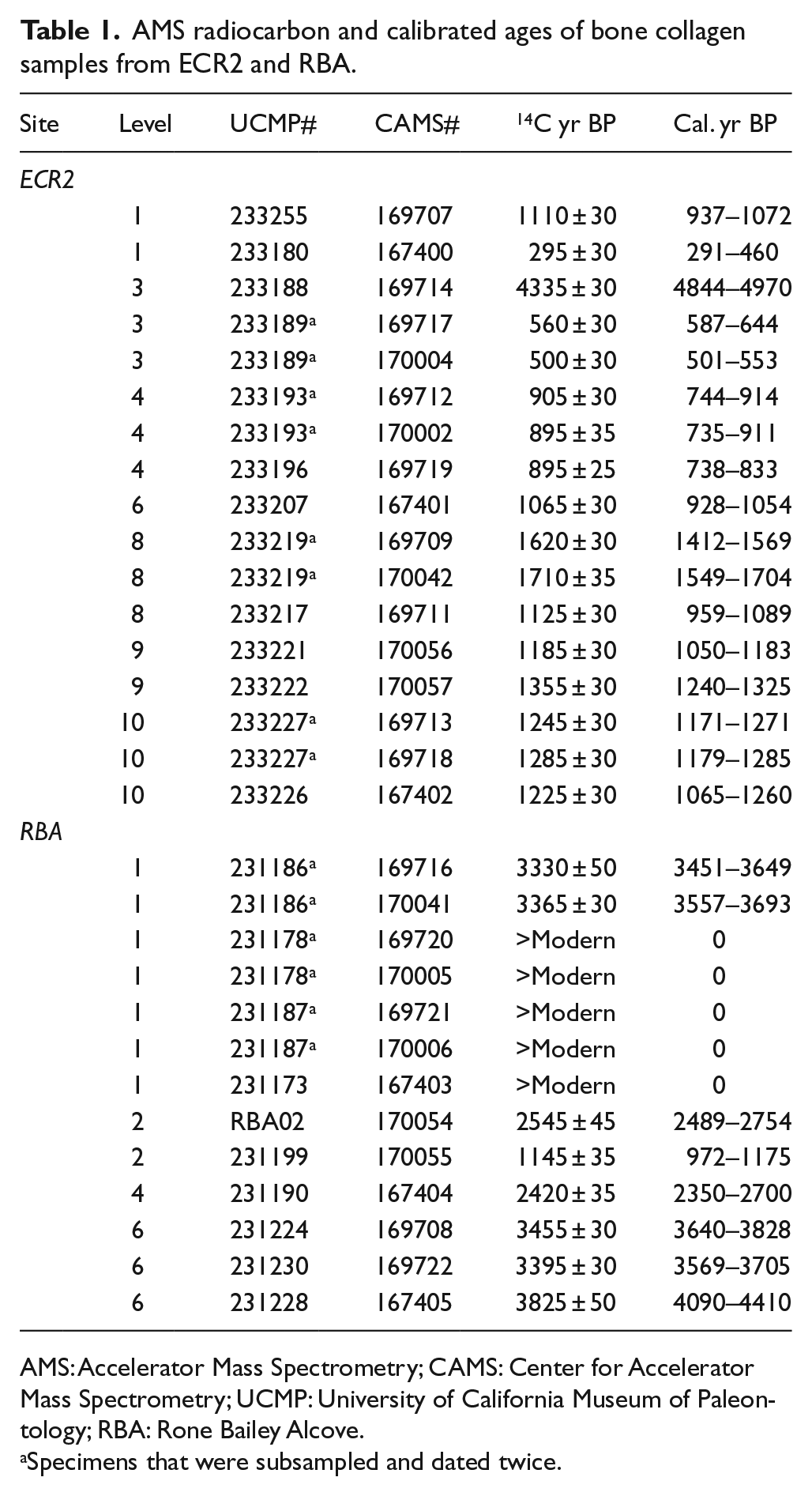
AMS: Accelerator Mass Spectrometry; CAMS: Center for Accelerator Mass Spectrometry; UCMP: University of California Museum of Paleontology; RBA: Rone Bailey Alcove.

Specimens that were subsampled and dated twice.

Faunal data for excavation levels with overlapping radiocarbon age ranges (Figure 2) were combined, and I developed a chronology of six time bins with different degrees of time averaging, dating from 4410 to 501 cal. BP.

Figure 2.

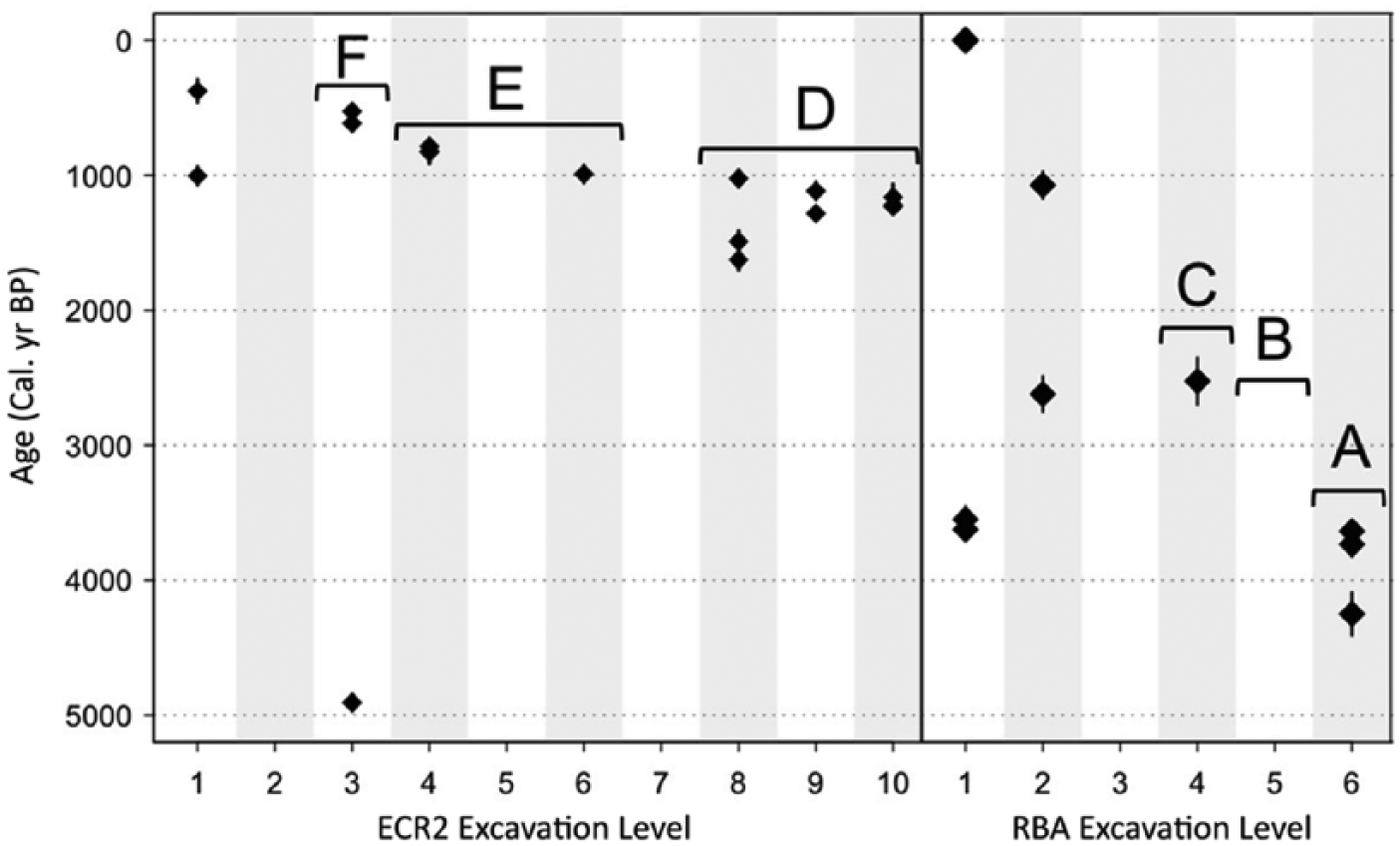
Calibrated age (cal. yr BP) of bone collagen samples from ECR2 and RBA. Diamonds indicate mean cal. yr BP, and vertical lines indicate the age range. Brackets indicate the excavation levels that were combined to produce time bins (letters).

Sample standardization

Taxon abundance was quantified as number of individual specimens (NISP) of craniodental material identified to family (Leporidae, Sciuridae), subfamily (Perognathinae, Arvicolinae), or genus (Onychomys, Cynomys, Dipodomys, Peromyscus, Neotoma, and Thomomys). As compared with minimum number of individuals (MNI), NISP has been demonstrated to be a less-biased indicator of relative importance of a taxon in the community (Blois et al., 2010; Grayson, 1978). Species-level identifications within these taxa are often only possible by comparison of skeletal elements that are seldom well represented in the fossil record. Analysis at taxonomic levels above the species level allows incorporation of more of the fossil data represented in these deposits, improving abundance estimations by increasing sample size. Furthermore, analysis at the genus, family, and subfamily levels provides the requisite information needed to recognize the relative changes in the small mammal taxa that fill different functional roles in the ecosystem (Barnosky, 2004; Barnosky et al., 2004; Blois et al., 2010; Grayson, 2000; Terry et al., 2011) and which can be used as appropriate metrics of the environmental state (Badgley and Fox, 2000; Barnosky and Shabel, 2005; Barnosky et al., 2004; Stegner and Holmes, 2013).

I calculated relative abundance as NISP of the taxon divided by the total number of specimens for each time bin. I then estimated 95% confidence intervals around each relative abundance estimate using Goodman’s (1965) simultaneous confidence interval calculations (Calede et al., 2011; McHorse et al., 2012), implemented in the DescTools package in R (Signorell et al., 2015).

Species richness is correlated with sample size, so I standardized richness using shareholder quorum subsampling (SQS) at a coverage level of 0.6 (Alroy, 2010). While the goal of traditional rarefaction is uniform sampling, the purpose of SQS is ‘fair’ sampling that is reflective of the true standing diversity. In SQS, sample size is not fixed; rather, SQS fixes coverage, the proportion of the entire frequency distribution represented by the species in the resample. Rarefaction dampens the richness of very diverse samples, so relative diversity estimates are not linear, whereas in SQS a site that is twice as diverse as another has an SQS richness value that is twice as large (Alroy, 2010). Estimated richness values produced by SQS appear low relative to raw richness, but are linearly proportional to one another.

Estimation of confidence intervals is one way to correct for differences in time bin duration, but longer time bins inevitably have more opportunity to sample more species, and low sample size, as in bins F and A, can lead to a randomly biased NISP and abundance distribution structure. I tested for a correlation between duration and both raw and standardized richness per time bin and found no relationship between the two (raw richness: Pearson’s product moment correlation = 0.017, p = 0.97; standardized richness: Pearson’s product moment correlation = –0.276, p = 0.60).

All analyses were performed using the R Project for Statistical Computing version 3.2.0 (R Core Team, 2015) and with the vegan package (Oksanen et al., 2015), DescTools package (Signorell et al., 2015), and SQS function (Alroy, 2010).

Analysis of diversity change

I assessed diversity change through time in several different ways. First, I used pairwise Fisher’s tests to compare the relative abundance distribution from one time bin to the next (with a Monte Carlo p-value simulation, 1000 replicates, and both with and without a Holm p-value correction). Second, I calculated Hurlbert’s probability of interspecific encounter (PIE) for each time bin and compared across time bins. PIE is a measure of species evenness and is independent of sample size, unlike many other commonly used diversity metrics, for example, Shannon and Simpson indices (Blois et al., 2010; Gotelli and Ellison, 2013; Hurlbert, 1971). Because PIE is not biased by sample size, resampling is not necessary for estimating the uncertainty in the metric. Instead, I followed the equation presented in Davis (2005) for computing variance in PIE. Because time bins are likely to be serially autocorrelated and therefore non-independent, I compared the overlap in variance to determine whether PIE was significantly different among time bins (Blois et al., 2010).

I visualized faunal relationships among time bins using non-metric multidimensional scaling (NMDS) of relative abundance data. Unlike other ordination techniques (e.g. principal components or principal coordinates analysis), NMDS does not preserve true distances between objects (time bins or taxa in this case) and instead uses rank order of the distances between objects to arrange them in multidimensional space. This technique places more different objects further apart and more similar objects closer together, which is not always the case in other ordination techniques (Gotelli and Ellison, 2013).

Rank-order abundance was scaled from 1 to 10, to account for time bins where not all species were represented or when some taxa had the same number of specimens. I made pairwise comparisons of rank-order abundance between time bins using Spearman rank correlation tests with and without a Holm p-value correction. The Spearman coefficient ranges from −1, indicating an inverse relationship, to 1, indicating perfect correspondence (Terry, 2010a). To determine whether particular taxa were consistently higher or lower in rank than the others, I compared the ranks of taxa using pairwise Mann–Whitney U-tests with and without Holm p-value corrections.

Climate correlation

To evaluate the role of climate across all six time bins, I used reconstructed mean July temperature (MJT) for the Southwestern United States from Viau et al. (2006), downloaded from the National Climatic Data Center (http://www.ncdc.noaa.gov). These reconstructions are based on 752 fossil and 4590 modern pollen records from across the continent and estimate MJT in 100-year intervals from 14 kyr to the present (Viau et al., 2006). Following the methods described in Terry and Rowe (2015) and Rowe and Terry (2014), I fit the climate data with a spline smoothing function (R function spline: stats, method: natural) and then analytically averaged the climate data over the period of time encompassed by each time bin. I then used cross-correlation to test for a relationship between climate and species richness, evenness, and relative and rank abundance of each taxon. The significance of the correlations was tested using permutation tests (500 iterations). To evaluate lagged correlations, I shifted the climate data by 10-year increments, up to 200 years, each time re-averaging the fitted climate data and recalculating the correlation (Terry and Rowe, 2015).

Results

Radiocarbon chronology

Radiocarbon chronologies for each site show that most dates were stratigraphically consistent, with levels ranging from 143 (ECR2 level 3) to 841 (RBA level 6) years of time averaging (Table 1, Figure 2). Dates presented in Figure 2 are derived from the most likely age for each specimen. However, there is a range of possible calibrated cal. BP for a given ¹⁴C date (Figure 2); I used the probability distribution associated with each date and the overlap in possible calibrated ages to determine which excavation levels could reasonably be considered non-overlapping in age. The three older time bins pertain to RBA, while the younger are from ECR2. Time bin A, the oldest, represents excavation level 6 from RBA and has peak age probabilities at 3699.5, 3639.5, and 4184.5 cal. BP. RBA level 5 was not dated, but dates for levels 6 and 4 are consistent and non-overlapping, so here I assume that stratigraphic mixing in these older layers is either not present or very minimal and that level 5 can be treated as a separate faunal unit (time bin B). However, additional radiocarbon dates are necessary to confirm this assumption. Level 4 encompasses time bin C with peak age probability at 2424.5 cal. BP. Time bin D represents ECR2 excavation levels 8–10, with peaks at 1024.5, 1169.5, 1179.5, 1194.5, 1214.5, 1289.5, 1529.5, and 1609.5 cal. BP. Time bin E represents ECR2 levels 4–6 and peaks at 794.5, 789.5, and 959.5 cal. BP. Time bin F is represented by ECR2 level 3. The oldest date from ECR2, 4970–4844 cal. BP, is from excavation level 3 and is ~2.6 kyr older than the next oldest date (from level 8). If this is excluded, bin F/level 3 has peaks at 524.5 and 544.5 cal. BP. While there is no evidence that this particularly old date is inaccurate, either as a result of contamination in the lab or in the deposit, these kinds of contamination are extremely difficult to diagnose. However, all other dates for ECR2 are consistently younger than 1704 cal. BP, and so this date of nearly 5 kyr in the middle of the deposit has a few important implications. First, it suggests that stratigraphic mixing is present to a certain degree in this site, but that it occurs rarely because dates from other levels tend to be consistent and arranged in a predictable chronological order. ECR2 level 1 and RBA levels 1 and 2 both have wider age ranges and show more mixing than the deeper/older excavation levels. Those levels have not been included in these analyses because the magnitudes of time averaging they encompass entirely overlap deeper excavation levels. ERC2 level 2 and RBA level 3 were not dated and were also excluded because it is not known whether they are highly mixed, and it appears that younger levels may be more mixed than older levels. Bioturbation by people, cattle, and rodents is one possible explanation for the presence of older bones in top excavation levels. Second, while there is some mixing in these sites, dates generally get older with increasing depth, suggesting it is reasonable to assume that the majority of the material in each level has not moved dramatically up or down in the deposit. Combining neighboring excavation levels into single analysis units helps to strengthen this assumption. However, interpretation of the age of individual specimens is not possible without a date on the specimen itself.

Relative and rank-order abundance

Abundance of taxa fluctuates across the record (Table 2, Figure 3), but 95% confidence intervals demonstrate that there is no significant difference in relative abundance through time within each taxon and few differences among taxa (Figure 3). In time bin A, observed relative abundances of arvicolines and Thomomys were at their highest, while leporids, perognathines, Cynomys, and Onychomys were not sampled at all. During B, leporids, perognathines, Cynomys, and Onychomys first appeared, and perognathines were at their most abundant across the record. Dipodomys also increased in abundance, while sciurids, arvicolines, Peromyscus, Neotoma, and Thomomys all declined. In bin C, leporids, Cynomys, Neotoma, Onychomys, Peromyscus, and arvicolines all increased, while sciurids, Thomomys, Dipodomys, and perognathines declined. Leporids and Cynomys continued to increase in bin D, along with slight increases in Neotoma, Onychomys, Peromyscus, and sciurids. Dipodomys and Thomomys continued to decline, Thomomys reaching its lowest abundance across the record, and arvicolines also decreased. Cynomys was again absent during bin E; Neotoma declined while Onychomys and Peromyscus slightly increased. After relatively low abundance in the preceding time bin, Thomomys sharply increased in E. Perognathines, Dipodomys, and sciurids also increased while leporids slightly declined. Bin F is characterized by extremes: leporids, Thomomys, and Neotoma were at their highest abundance, but Onychomys, Cynomys, and arvicolines were entirely absent. Dipodomys declined slightly, and Peromyscus, sciurids, and perognathines maintained low abundance.

Table 2.

Number of individual specimens (NISP) (above) with relative abundance (taxon NISP/total NISP) and 95% Goodman’s simultaneous confidence intervals (italics) (below); uncorrected species richness and standardized (SQS) richness.

Taxon	A	B	C	D	E	F
Arvicolinae	1	1	4	1	2	0
	0.08 (0–0.63)	0.01 (0–0.2)	0.05 (0.01–0.24)	0.02 (0–0.28)	0.01 (0–0.13)	0 (0–0.3)
Cynomys	0	1	2	3	0	0
	0 (0–0.57)	0.01 (0–0.2)	0.02 (0–0.2)	0.06 (0.01–0.33)	0 (0–0.1)	0 (0–0.3)
Dipodomys	4	35	30	11	32	6
	0.31 (0.05–0.78)	0.45 (0.25–0.67)	0.35 (0.18–0.57)	0.22 (0.07–0.5)	0.22 (0.11–0.38)	0.15 (0.03–0.48)
Leporidae	0	3	4	12	22	11
	0 (0–0.57)	0.04 (0.01–0.24)	0.05 (0.01–0.24)	0.24 (0.08–0.52)	0.15 (0.07–0.31)	0.28 (0.09–0.6)
Neotoma	1	4	10	6	11	5
	0.08 (0–0.63)	0.05 (0.01–0.25)	0.12 (0.04–0.33)	0.12 (0.03–0.4)	0.08 (0.02–0.22)	0.13 (0.03–0.46)
Onychomys	0	2	7	2	9	0
	0 (0–0.57)	0.03 (0–0.22)	0.08 (0.02–0.28)	0.04 (0–0.3)	0.06 (0.02–0.2)	0 (0–0.3)
Perognathinae	0	5	3	0	5	1
	0 (0–0.57)	0.06 (0.01–0.27)	0.04 (0–0.22)	0 (0–0.25)	0.03 (0.01–0.16)	0.03 (0–0.34)
Peromyscus	1	3	7	4	20	1
	0.08 (0–0.63)	0.04 (0.01–0.24)	0.08 (0.02–0.28)	0.08 (0.01–0.35)	0.14 (0.06–0.29)	0.03 (0–0.34)
Sciuridae	1	6	2	8	3	3
	0.08 (0–0.63)	0.08 (0.02–0.29)	0.02 (0–0.2)	0.16 (0.04–0.44)	0.02 (0–0.14)	0.08 (0.01–0.4)
Thomomys	5	18	16	4	42	12
	0.38 (0.08–0.82)	0.23 (0.09–0.46)	0.19 (0.07–0.41)	0.08 (0.01–0.35)	0.29 (0.16–0.46)	0.31 (0.11–0.63)
Uncorrected richness	6	10	10	9	9	7
SQS richness	2.567	2.261	3.183	3.97	3.972	2.712

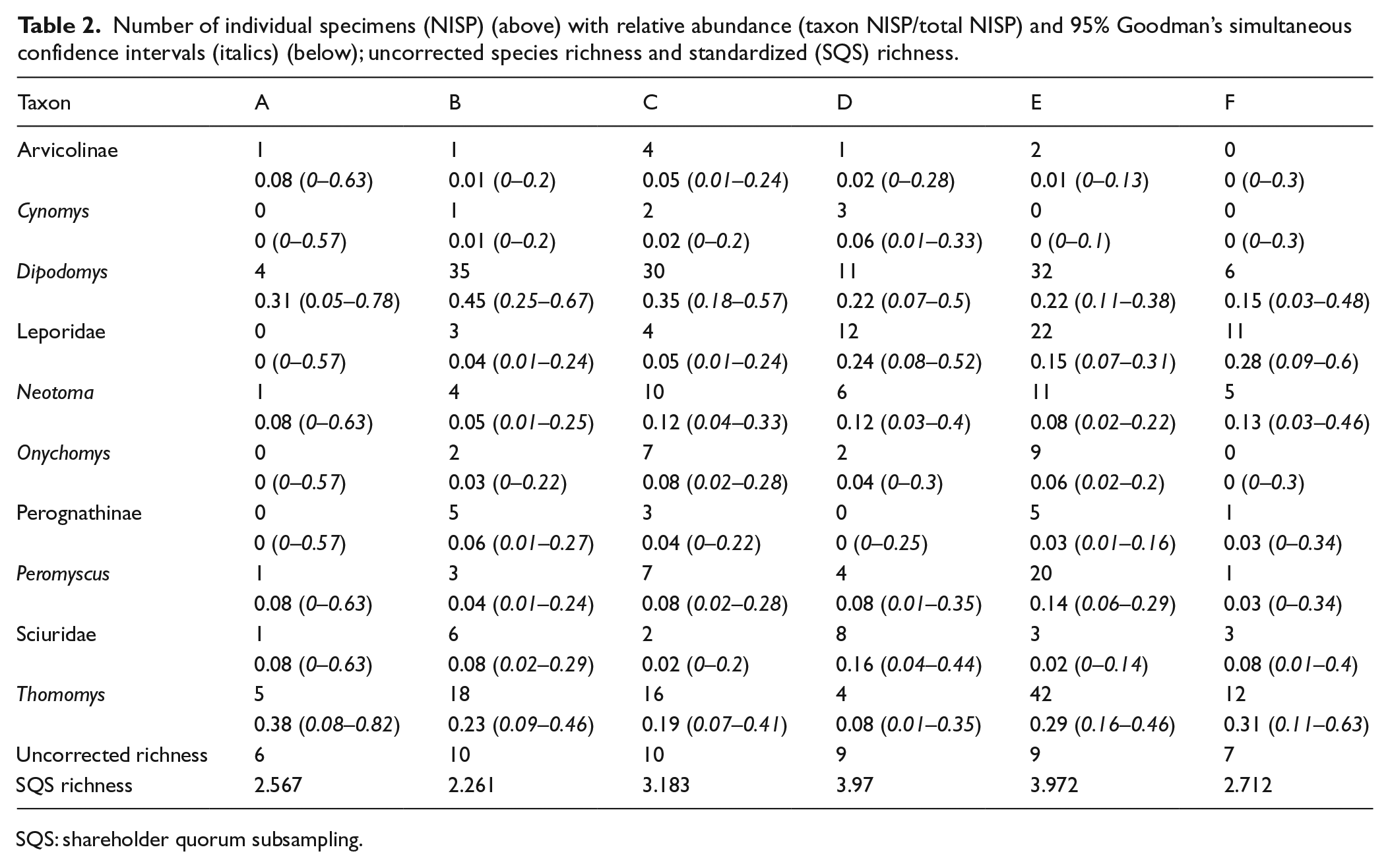
SQS: shareholder quorum subsampling.

Figure 3.

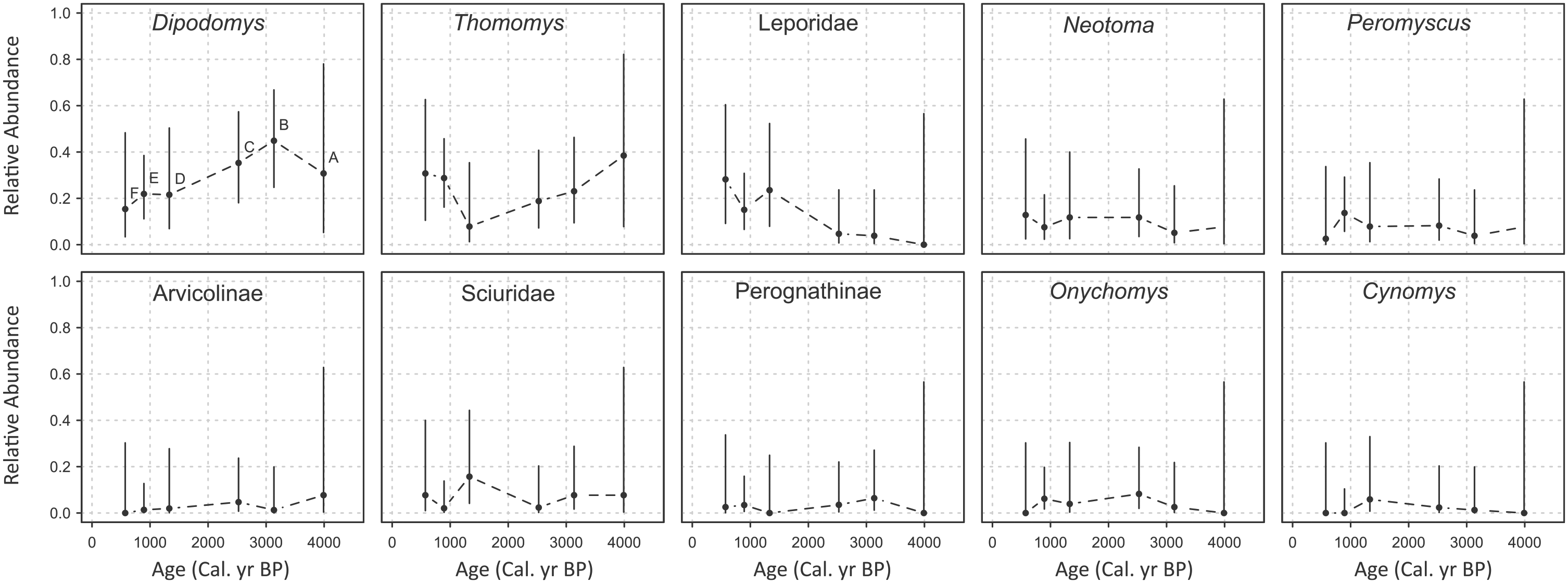
Relative abundance of each taxon through time. Vertical bars are Goodman’s simultaneous 95% confidence intervals. The order of time bins is illustrated for Dipodomys only; the same order applies for all taxa.

The rank-order abundances are all positively correlated across time bins (Figure 4, Table 3). Without the Holm p-value correction for multiple statistical tests, the rank-order abundances of B, E, and F are significantly correlated with one another; additionally, C is correlated with A and E, and D is correlated with F. All of these comparisons have correlation coefficients over 0.60. With a Holm correction, only E versus C and F versus E are significantly correlated. The Mann–Whitney U-tests (Table 4, Figure 4) show that, without a p-value correction, Dipodomys and Thomomys are significantly more rank abundant (more common taxa have lower rank abundance values; that is, rank of 1 is the first most common taxon) than all taxa except for leporidae and Neotoma (only Dipodomys is significantly higher in rank than Neotoma). Arvicolines are significantly less rank abundant than all other taxa except for Onychomys, perognathines, and sciurids; Cynomys is significantly less rank abundant than all taxa except Onychomys, perognathines, and arvicolines. No comparisons are significant when a Holm p-value correction is used.

Figure 4.

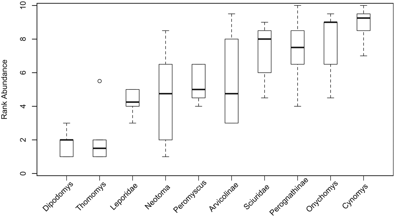
Boxplot of rank-order abundance ranks across time bins for each taxon.

Table 3.

Correlation coefficients from pairwise Spearman rank correlation tests on rank-order abundance of taxa for each time bin (above); Fisher’s test uncorrected p-values, for pairwise comparison of abundance distribution among time bins (below, in italics).

	A	B	C	D	E
B	0.62
	0.54
C	0.65*	0.46
	0.41	0.08
D	0.32	0.46	0.29
	0.00 *	0.01 *	0.00 **
E	0.52	0.64*	0.81*	0.55
	0.72	0.30	0.11	0.08
F	0.53	0.76*	0.51	0.73*	0.82**
	0.63	0.05 *	0.29	0.01 *	0.49

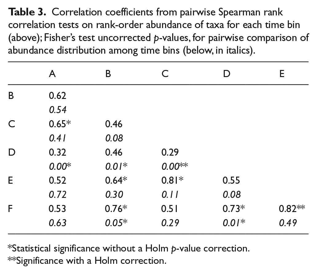
Statistical significance without a Holm p-value correction.

Significance with a Holm correction.

Table 4.

The p-values from pairwise Mann–Whitney tests.

	Dipodomys	Thomomys	Neotoma	Leporidae	Peromyscus	Sciuridae	Onychomys	Perognathinae	Arvicolinae
Dipodomys (1.83)
Thomomys (2.08)	0.796
Neotoma (4.25)	0.006*	0.062
Leporidae (4.58)	0.117	0.100	1.000
Peromyscus (5.25)	0.005*	0.023*	0.166	0.806
Sciuridae (5.50)	0.007*	0.029*	0.625	0.572	0.936
Onychomys (7.33)	0.005*	0.008*	0.016	0.147	0.063	0.257
Perognathinae (7.33)	0.005*	0.008*	0.029	0.106	0.075	0.261	1.000
Arvicolinae (7.92)	0.004*	0.007*	0.015*	0.042*	0.041*	0.168	0.288	0.518
Cynomys (8.92)	0.005*	0.005*	0.005*	0.010*	0.005*	0.043*	0.064	0.147	0.325

Significance without a Holm correction. No pairwise comparisons were significant with a Holm correction. Mean rank for each taxon is in parentheses.

Diversity dynamics

The abundance distribution of bin D was significantly different (Fisher’s test without p-value correction) from all time bins except E (Table 3). Bins B and F were also significantly different from one another. NMDS (Figure 5) illustrates the relative degree of compositional similarity among time bins, although no time bins form tight groups with one another. Sample size is low in bins A (n = 13) and F (n = 39), which could have a meaningful impact on the results of the Fisher’s tests and on the arrangement of time bins and taxa in the NMDS.

Figure 5.

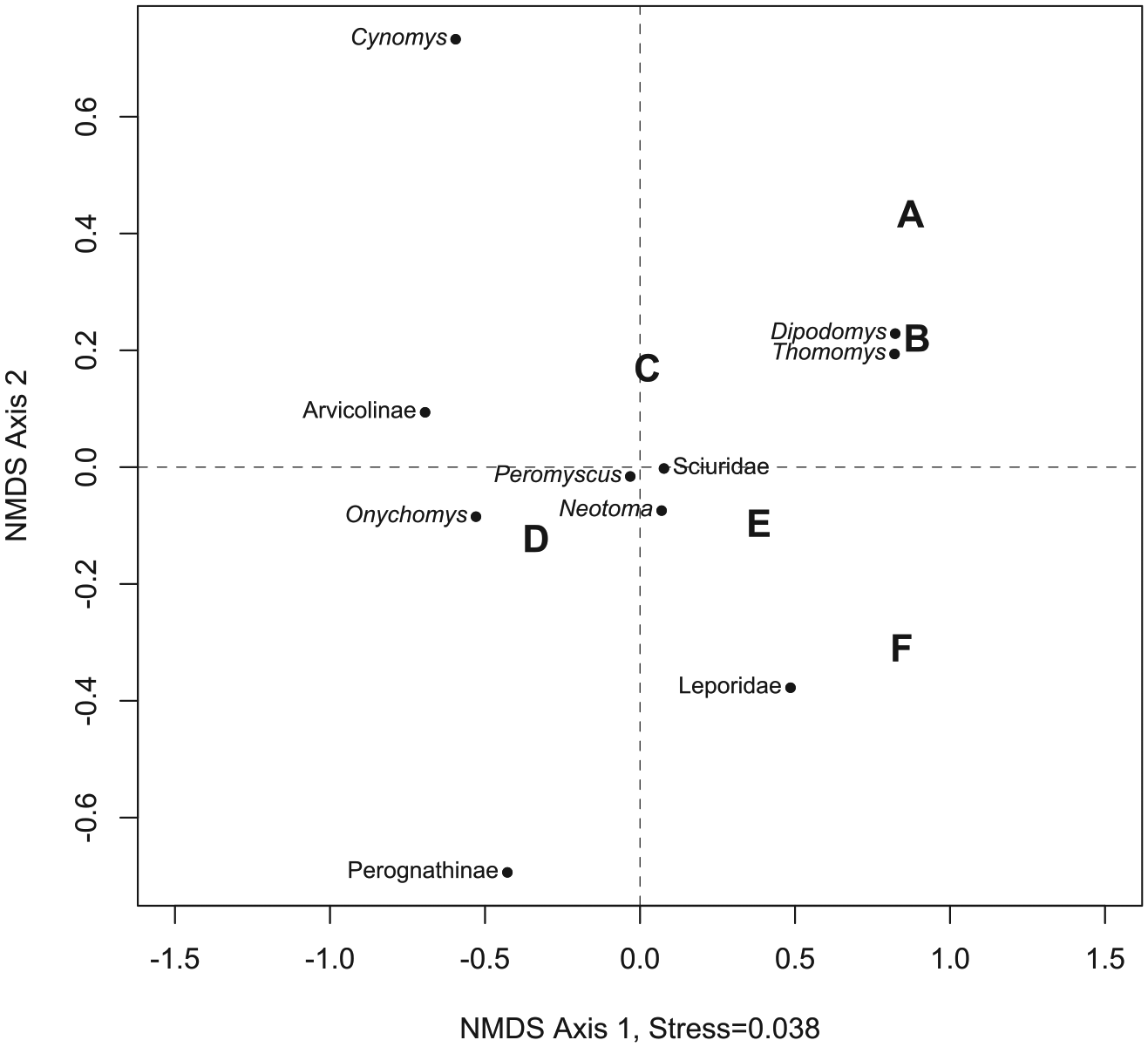
Plot of non-metric multidimensional scaling of relative abundance.

PIE (Figure 6) was relatively high in time bins A (4410–3569 cal. BP), C (estimated 2700–2350 yr. BP), E (1054–735 cal. BP), and F (644–501 cal. BP). It reached a peak during bin D (1704–959 cal. BP), but was significantly lower than other times during bin B (3569–2700 cal. BP). Variance is non-overlapping for all time bins, except A and F overlap.

Figure 6.

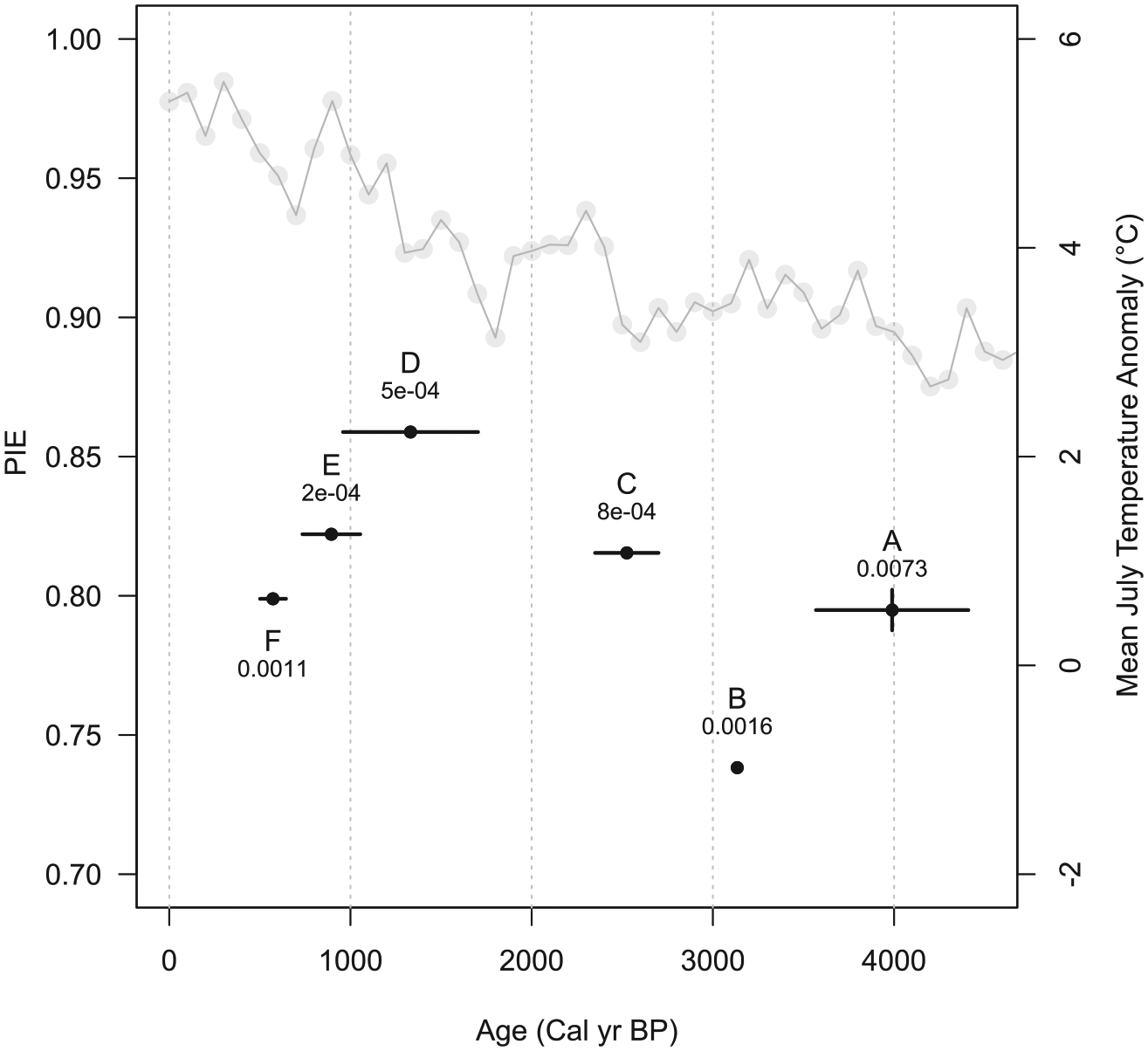
PIE index for each time bin; vertical black bars and numbers are the variance associated with each PIE value. Letters indicate time bin and horizontal black bars are the age range (cal. yr BP). Time bin B was not dated, so the age range is unknown. The gray line and points are reconstructed mean July temperature anomaly from Viau et al. (2006).

Climate correlations

There were no significant correlations between MJT and diversity using temporal cross-correlation except for relative abundance of leporids, which had the highest correlation coefficient at lag = 0 (r = 0.83, p = 0.026). Because sample sizes are low, particularly in bins A and B, there is high degree of uncertainty around the relative abundance of each taxon, illustrated in Figure 3. Additional specimens could change these results by changing the relative abundance distribution for each time bin. Additional specimens are more likely to change the rank abundance for less common taxa (ranks above 3) because the magnitude of difference in NISP is smaller among the less common taxa than among the most common taxa. In short, larger sample size is unlikely to change the fact that Dipodomys, Thomomys, and leporids are generally the most common taxa.

Discussion

Overall, neither diversity nor abundance in ECR2 and RBA correlates with the climate record assessed here. There were no significant differences in abundance of taxa throughout the record, from ~4.4 to 0.5 kyr. Most of the taxa present in these deposits are tolerant or characteristic of xeric ecosystems, and only one taxon present in the fossil record is not found in the immediate vicinity of the caves today (voles, genus Lemmiscus and Microtus).

Species of Microtus are typically found in grasslands and meadows, often associated with montane and/or riparian ecosystems (Kays and Wilson, 2009). In the fossil record, Microtus tends to be associated with cooler and more mesic times (Barnosky, 2004; Hadly, 1996; Hadly and Barnosky, 2009). In contrast, the sagebrush vole, Lemmiscus curtatus, is found in more arid brushy environments – usually sagebrush or rabbit brush (Carroll and Genoways, 1980). L. curtatus is restricted to the Great Basin today but is found in late Pleistocene records from across the CP (Mead et al., 2003; Murray et al., 2005). Teeth of L. curtatus are present in ECR2 level 4 (time bin E, 1054–735 cal. BP) and RBA level 4 (time bin C, estimated 2700–2350 ybp). To my knowledge, these are the youngest records of L. curtatus on the CP (Bell and Glennon, 2003; Carrasco et al., 2005; FAUNMAP Working Group, 1994, 1996; Mead et al., 2003; Neotoma Paleoecological Database, 2013): other occurrences of this species on the CP in the last 40 kyr are Sheep Camp Shelter (late Glacial/Holocene; Gillespie, 1985), Screaming Neotoma Cave (29–25 kyr; Bell and Glennon, 2003; Mead et al., 2003), and Isleta Cave No. 2 (late Glacial/Holocene; Harris and Findley, 1964).

As MJT increased, leporid relative abundance also increased. However, the 95% confidence intervals around relative abundance of leporids overlap for all time bins, so it is possible that the observed increase is a sampling artifact. Sylvilagus and Lepus are both ubiquitous across the CP and in western North America generally and, as genera, are tolerant of a wide range of habitats (Kays and Wilson, 2009). In a study of Chihuahuan Desert Lepus californicus, Hernández et al. (2011) found a correlation between leporid abundance and both precipitation and plant productivity, and conclude that food supply has a strong effect on L. californicus abundance. In contrast, Lightfoot et al. (2010) also assessed leporid abundance dynamics in the Chihuahuan Desert but found no correlation between Sylvilagus audubonii or L. californicus abundance and precipitation or productivity. Rather, Lightfoot et al. (2010) observed higher diversity of both species in black gramma grassland as compared with creosote bush shrubland. L. californicus favors areas with sparse grass and vegetation cover, including heavily grazed areas, but avoids tall grasses and forests (Best, 1996). In contrast, the species of Sylvilgaus present in southeastern Utah today (S. audubonii and Sylvilagus nuttali) are more commonly associated with brushy areas (Chapman, 1975; Chapman and Willner, 1978). It is not generally possible to distinguish Lepus from Sylvilagus using morphological criteria or size of loose teeth (Robinson and Matthee, 2005; Stegner, 2015), so it is unclear whether the increase in leporids in RBA and ECR2 is driven by one genus or whether both became more abundant through time. Climate was almost certainly becoming more arid at these sites after about 2 kyr (Cook and Krusic, 2004; Pederson et al., 2011; Reheis et al., 2005) and local changes in the plant community were likely taking place, which may have favored leporids. Identification of the pollen from these sites would shed light on this question.

A second pattern is qualitatively evident in the relative abundance data (Table 2): when Thomomys have lower relative abundance, Neotoma and Peromyscus are higher in abundance. Also, as Dipodomys declines through time, leporids increase. However, Dipodomys and Thomomys remain the most common (first and second most abundant, respectively) throughout the record, except bin D (leporids are first in rank abundance, Dipodomys are second, and Thomomys are fifth) and bin F (Thomomys are first, leporids are second, and Dipodomys are third). Terry et al. (2011) found that granivores tended to increase in abundance as climate warmed: of the two granivores at ECR2 and RBA, Dipodomys actually decline in abundance as climate warmed, and perognathines appear to fluctuate at low abundance independently of climate. Abiotic affinities do not seem to be related to this relative abundance pattern: Dipodomys are physiologically adapted to dry environments (Vimtrup and Schmidt-Nielsen, 2005) and are found in a range of arid and semi-arid habitats (Garrison and Best, 1990; Kays and Wilson, 2009); Dipodomys ordii, the only species found in northern San Juan County today, is almost always associated with sandy soils (Garrison and Best, 1990). The two species of Thomomys present in Utah today are Thomomys talpoides, found generally in the mountains and high valleys of Utah (Durrant, 1952), and Thomomys bottae, generally found in agricultural fields (such as alfalfa), lower valleys, and desert mountains (Durrant, 1952; Verts and Carraway, 1999). However, both have extremely wide geographic, elevational, and ecological ranges (Durrant, 1952; Jones and Baxter, 2004; Verts and Carraway, 1999), and so their present-day distribution in Utah is not necessarily a good indicator of their fossil distribution or habitat preferences.

Peromyscus and Neotoma are also fairly generalist in their climatic requirements and are dietary generalists as well (Blois et al., 2010; Sorensen et al., 2004). Certain species within these genera are specialists, however – for example, Peromyscus truei (pinyon mouse) is found associated with pinyon (Hoffmeister, 1981), and Neotoma stephensi is associated with juniper or, occasionally, other conifers (Sorensen et al., 2004). Finer taxonomic resolution of the fossil data would certainly aid in interpretation of abundance dynamics, for example, by revealing intra-generic turnover, but isolated teeth of Peromyscus and Neotoma cannot be identified to species using standard morphological criteria (Grayson, 1988; Hooper, 1957; Mead and Phillips, 1981; Mead et al., 2003; Repenning, 2004; Stegner, 2015). Using the dental morphological criteria developed by Hooper (1957), I attempted to identify Peromyscus teeth from ECR2 and RBA to species. However, almost all teeth were morphologically aligned with at least two of four species present in this region today: Peromyscus maniculatus, Peromyscus crinitus, Peromyscus boylei, and P. truei (Supplemental 3, available online).

The few sciurid specimens from ECR2 and RBA are almost exclusively loose cheek teeth, and the high degree of wear on these teeth makes identification to genus challenging, with the exception of Cynomys which is more hypsodont than other sciurids and larger than all other sciurids except Marmota. Today, the sciurids present in southeastern Utah include the burrowing Cynomys gunnisoni, Ammospermophilus leucurus (white-tailed antelope squirrel), Otospermophilus variegatus (rock squirrel), and Xerospermophilus spilosoma (spotted ground squirrel); largely ground-dwelling Tamias mimimus (least chipmunk), Tamias quadrivitattus (Colorado chipmunk), and Tamias rufus (Hopi chipmunk); and tree-dwelling Sciurus aberti (Abert’s squirrel). All of these species, with the exception of S. aberti, are found in arid desert and scrubland habitats today (Belk and Smith, 1991; Best et al., 1994; Burt and Best, 1994; Kays and Wilson, 2009; Nash and Seaman, 1977; Oaks et al., 1987; Streubel and Fitzgerald, 1978; Verts and Carraway, 2001). I have trapped both Tamias and Ammospermophilus in patches of pinyon–juniper woodland near these sites. S. aberti is present in the Abajos today (Schaefer, 1991) but not outside montane, forested regions (Kays and Wilson, 2009) – the presence of S. aberti in the fossil record of ECR2 and RBA might indicate cool/mesic climatic conditions. The sciurid teeth recovered from ECR2 and RBA are likely too small to be Sciurus, but further research will be necessary to confirm. The Cynomys recovered from RBA and ECR2 are white-tailed prairie dogs, subgenus Leucocrossuromys, which still persist less than 1 km southeast of ECR2 today. Cynomys, even on a subgenus-level, is unlikely to be a good indicator of climate: prairie dogs can persist in semi-desert (C. (L.) leucurus), grasslands and prairies (C. (L.) parvidens, C. (C.) ludovicianus), as well as montane meadows (C. (L.) gunnisoni, C. (L.) leucurus) (Kays and Wilson, 2009).

Two additional arid-adapted taxa are present throughout the deposits in relatively low abundance. Today, perognathines – genus Perognathus and Chaetodipus – are generally found in arid or semi-arid grasslands, desert scrub, or shrub steppe, but several species also occupy woodlands and chaparral (Kays and Wilson, 2009). Only Perognathus is present on the CP today. Onychomys also occupies arid and semi-arid regions of North America: Onychomys leucogaster, the only species currently found on the CP, prefers shrub steppes and grasslands (McCarty, 1975, 1978). O. leucogaster can be distinguished from its only sister species, Onychomys torridus – found in the Sonoran and part of the Chihuahuan Deserts – using length and width dimension of the m1 and m3 (Carleton and Eshelman, 1979). However, because there is overlap in the measurements for these species (Carlton and Eshelman, 1979), a sample size larger than what is available at ECR2 and RBA is required. Furthermore, many mammal species change their body size in response to climate (Smith and Betancourt, 1998), so morphological criteria are preferable to size for making identifications (Bell et al., 2010).

Taxa with similar relative abundance dynamics group closer together in the NMDS results (Figure 5). Two close taxonomic groups are evident: (1) Dipodomys and Thomomys (highest rank-order abundance across the record, higher relative abundance in the beginning and end of the record, lower in the middle), and (2) Neotoma, Peromyscus, and sciurids (higher in the beginning, then an early dip in abundance followed by an increase, then yet another dip). These groupings do not seem to be connected to climatic affinity because a mixture of taxa with xeric, mesic, or neutral affinity is found in each grouping and abundance does not correlate with MJT.

Desert taxa might be expected to respond more to aridity than to temperature (Stapp, 2010). Several lines of evidence indicate that conditions were relatively cool and wet during time bins A–C and then more arid and warm during D–F (Anderson et al., 2000; Betancourt, 1984; Betancourt and Davis, 1984; Coats et al., 2008; Reheis et al., 2005). Bins E and F encompass a period of time when at least six ‘megadroughts’ took place, including the droughts that are thought to have dispersed the Ancestral Puebloans at Chaco, Mesa Verde, Kayenta, and other large CP settlements (Benson and Berry, 2009; Benson et al., 2007). However, time bins with more similar climate (A–C vs D–F) do not group together on the NMDS, supporting the conclusion that relative and rank-order abundance dynamics are disconnected from climate, at least with regard to the broad-scale trends discussed here. One possible explanation is that time-averaged stratigraphic layers capture short cool or mesic periods within an overall aridifying and warming trend (Hadly, 1996). However, sample sizes for these cool/mesic taxa should be lower than for warm/xeric taxa if taphonomic processes are the same during wet and dry times.

Evenness, as measured using the PIE index, is not significantly correlated with climate. PIE is notably low during bin B (estimated 3569–2700 BP; cool and possibly more wet). At that time, relative abundance of Dipodomys was extremely high, and Neotoma and Peromyscus were at their lowest abundance. Evenness reached a peak in time bin D, when the three most common taxa (Dipodomys, Thomomys, and leporids) all had average relative abundance. Although the uncertainly around PIE does not overlap for most time bins, the magnitude of evenness change is low – from a maximum PIE of 0.85 in D to a minimum of 0.73 in B, a change of only 0.12 – supporting the conclusion that small mammal abundance at these sites was not detectably altered by the changes in climate that occurred during the interval of deposition.

Other factors not tested in this study, like Ancestral Puebloan population size and land use, may influence small mammal diversity dynamics. However, Fisher’s tests reveal that only time bin D was significantly different from the others in terms of the relative abundance distribution across the record. Furthermore, the taxonomic and functional components of this community have not changed markedly through the environmental changes represented by the time sampled by the deposits, suggesting that these groups persist despite natural variation and/or external perturbation in this system. However, finer taxonomic resolution might reveal a signature of climate change: for example, Thomomys subgenus Megascapheus is present in ECR2 and RBA throughout the time period encompassed by this study, but the only specimen of Thomomys subgenus Thomomys is from ECR2 level 3 (time bin F, 644–501 cal. BP). T. subgenus Thomomys is better able to burrow in harder soils than T. subgenus Megascapheus, and soils tend to get harder as climate dries (Marcy et al., 2013). While Thomomys abundance has remained high relative to other taxa for thousands of years, species and subspecies of Thomomys naturally replace one another as climate changes (Hadly and Barnosky, 2009).

Greater sample sizes at RBA and ECR2, particularly at the beginning and end of the record (time bins A and F), could alter the observed abundance patterns and might reveal a correlation between diversity and climate. However, the results reported here are in keeping with other studies of small mammal dynamics through the Holocene in western North America. For example, at Samwell Cave in northern California, Blois et al. (2010) found that small mammal evenness and richness dropped during the Pleistocene–Holocene transition, but during the last ~5 kyr both measures of diversity were fairly stable. At Homestead Cave in northern Utah, Terry and Rowe (2015) showed that energy dynamics, in terms of which small mammal guilds are dominant, changed dramatically at the end of the Pleistocene and again in the last century, but were stable throughout the Holocene. In contrast, Rowe and Terry (2014) compared small mammal diversity dynamics in Homestead Cave and Two Ledges Chamber, a site in northern Nevada, and demonstrated that during the same time interval (8 kyr to the present), species that were shared between sites had entirely different relative abundance dynamics. This suggests that local conditions may have a larger influence on relative abundances at a site than does regional climate (Stegner, 2015).

Conclusion

Two newly excavated late Holocene fossil midden localities, ECR2 and RBA, with 33 AMS ¹⁴C dates provide fine-resolution information on small mammal diversity dynamics from ~4.4 to 0.5 kyr in southeastern Utah. These sites comprise a chronology of six time bins. Regional temperature increased across the record, and ‘megadroughts’ marked the time period from ~1100 to 350 BP. I tested for an effect of temperature on community evenness and abundance of 10 small mammal taxa: leporids, perognathines, small sciurids, arvicolines, Cynomys, Neotoma, Dipodomys, Onychomys, Peromyscus, and Thomomys. Despite increases in temperature, measured as reconstructed MJT anomaly, neither is significantly correlated with relative abundance, rank abundance, species richness, or the PIE evenness index. Although abundance does not correlate with climate, certain groups of species have similar diversity trends through time. Identifying what drives these cross-taxa abundance patterns will be important for predicting future abundance changes.

Overall, these results indicate that climatic fluctuations of the magnitude preserved in these deposits do not significantly alter the small mammal community at least on the taxonomic level assessed here. Neither is there evidence that the presence, then exodus, of Native Americans in the region significantly affected small mammals. This lends support to the findings of other studies, like Terry and Rowe (2015), that small mammal communities of western North America were stable throughout the Holocene, but have undergone dramatic changes in structure in the last 100 years as a result of human activities leading to large-scale land cover changes, like invasive annual grasses. The metrics of community structure assessed here can be monitored in the modern small mammal community of this region: if these metrics are significantly different today or in the future from those seen in the fossil record, it may indicate anthropogenic influences outside the range of natural variability.

Footnotes

Acknowledgements

Thanks to AD Barnosky, AR Byrne, EB Davis, EA Hadly, DR Lindberg, and JL Patton for helpful discussion and training. I thank D Erwin, M Goodwin, P Holroyd, and C Marshall of the University of California Museum of Paleontology (UCMP) for curatorial and museum support; T Guilderson and P Zermeno for radiocarbon dating training and assistance; undergraduate assistants M Hardesty-Moore, P Garcialuna, H Bhullar, and P Uppal for processing midden matrix; R Hunt-Foster for assistance with permitting; and the Canyonlands Research Center, Nature Conservancy of Utah, and Redd Family of the Dugout Ranch for support in the field.

Funding

I am grateful to the following sources for funding this research: the Canyonlands Natural History Association, UC Berkeley Department of Integrative Biology, Sigma Xi, Sigma Xi-Berkeley Chapter, the Paleontological Society, the Geological Society of America, the UC Museum of Paleontology, Kappy Wells and the TIDES Foundation, and NSF GRFP Grant DGE-1106400.

References

Alroy

(2010) Fair sampling of taxonomic richness and unbiased estimation of origination and extinction rates. In: Alroy

Hunt

(eds) Quantitative Methods in Paleobiology (Paleontological society papers 16). Boulder, CO: Paleontological Society, pp. 55–80.

Anderson

(1993) A 35,000 year vegetation and climate history from Potato Lake, Mogollon Rim, Arizona. Quaternary Research 40: 351–359.

Anderson

Betancourt

Mead

. (2000) Middle- and late-Wisconsin paleobotanic and paleoclimatic records from the southern Colorado Plateau, USA. Palaeogeography, Palaeoclimatology, Palaeoecology 155: 31–57.

Anderson

Hasbargen

Koehler

(1999) Late Wisconsin and Holocene subalpine forests of the Markagunt Plateau of Utah, southwestern Colorado Plateau, U.S.A. Arctic, Antarctic, and Alpine Research 31: 366–378.

Badgley

Fox

(2000) Ecological biogeography of North American mammals: Species density and ecological structure in relation to environmental gradients. Journal of Biogeography 27: 1437–1467.

Barnes

(1993) Geology of the Moab Area. Moab, UT: Canyon Country Publications.

Barnosky

(2004) Faunal dynamics of small mammals through the Pit sequence. In: Barnosky

(ed.) Biodiversity Response to Climate Change in the Middle Pleistocene. Berkeley, CA: University of California Press, pp. 318–326.

Barnosky

Shabel

(2005) Comparison of mammalian species richness and community structure in historic and mid-Pleistocene times in the Colorado Rocky Mountains. Proceedings of the California Academy of Sciences 56: 50–61.

Barnosky

Bell

Emslie

(2004) Exceptional record of mid-Pleistocene vertebrates helps differentiate climatic from anthropogenic ecosystem perturbations. Proceedings of the National Academy of Sciences of the United States of America 101: 9297–9302.

10.

Belk

Smith

(1991) Ammospermophilus leucurus. Mammalian Species 368: 1–8.

11.

Bell

Glennon

(2003) Arvicoline rodents from Screaming Neotoma Cave, Southern Colorado Plateau, Apache County, Arizona, with comments on the Pleistocene biogeography of Lemmiscus curtatus. In: Schubert

Mead

Graham

(eds) Ice Age Cave Faunas of North America. Bloomington, IN: Indiana University Press, pp. 34–63.

12.

Bell

Gauthier

Bever

(2010) Covert biases, circularity, and apomorphies: A critical look at the North American Quaternary Herpetofaunal Stability Hypothesis. Quaternary International 271: 30–36.

13.

Belnap

(2003) Biological soil crusts in deserts: A short review of their role in soil fertility, stabilization, and water relations. Algological Studies 109: 113–126.

14.

Belnap

Reynolds

Reheis

(2009) Sediment losses and gains across a gradient of livestock grazing and plant invasion in a cool, semi-arid grassland, Colorado Plateau, USA. Aeolian Research 1: 27–43.

15.

Benson

Berry

(2009) Climate change and cultural response in the prehistoric American Southwest. KIVA: The Journal of Southwestern Anthropology and History 75: 89–119.

16.

Benson

Peterson

Stein

(2007) Anasazi (pre-Columbian Native-American) migrations during the middle-12^th and late-13^th centuries – Were they drought induced? Climate Change 83: 187–213.

17.

Best

(1996) Lepus californicus. Mammalian Species 530: 1–10.

18.

Best

Burt

Bartig

(1994) Tamias quadrivittatus. Mammalian Species 466: 1–7.

19.

Betancourt

(1984) Late Quaternary plant zonation and climate in southeastern Utah. Great Basin Naturalist 44: 1–35.

20.

Betancourt

Davis

(1984) Packrat middens from Canyon de Chelly, Northeastern Arizona: Paleoecological and archaeological implications. Quaternary Research 21: 56–64.

21.

Blois

McGuire

Hadly

(2010) Small mammal diversity loss in response to Pleistocene climate change. Nature 465: 773–775.

22.

Bronk Ramsey

(2009) Bayesian analysis of radiocarbon dates. Radiocarbon 51: 337–360.

23.

Brown

Nelson

Vogel

(1988) Improved collagen extraction by modified Longin method. Radiocarbon 30: 171–177.

24.

Burt

Best

(1994) Tamias rufus. Mammalian Species 460: 1–6.

25.

Calede

JJM

Hopkins

SSB

Davis

(2011) Turnover in burrowing rodents: The roles of competition and habitat change. Palaeogeography, Palaeoclimatology, Palaeoecology 311: 242–255.

26.

Carleton

Eshelman

(1979) A synopsis of fossil grasshopper mice, genus Onychomys, and their relationships to recent species. The University of Michigan Museum of Paleontology Papers on Paleontology 21: 1–63.

27.

Carrasco

Kraatz

Davis

. (2005) Miocene Mammal Mapping Project (MIOMAP). University of California Museum of Paleontology. Available at: http://www.ucmp.berkeley.edu/miomap/.

28.

Carroll

Genoways

(1980) Lagurus curtatus. Mammalian Species 124: 1–6.

29.

Chapman

(1975) Sylvilagus nuttali. Mammalian Species 56: 1–3.

30.

Chapman

Willner

(1978) Sylvilagus audubonii. Mammalian Species 106: 1–4.

31.

Chronic

(1990) Roadside Geology of Utah. Missoula, MT: Mountain Press Publishing Company.

32.

Coats

Cole

Mead

(2008) 50,000 years of vegetation and climate history on the Colorado Plateau, Utah and Arizona, USA. Quaternary Research 70: 322–338.

33.

Cole

(1990) Reconstruction of past desert vegetation along the Colorado River using packrat middens. Palaeogeography, Palaeoclimatology, Palaeoecology 76: 349–366.

34.

Conservation Paleobiology Workshop (2012) Conservation paleobiology: Opportunities for the earth sciences. Report, Division of Earth Sciences, National Science Foundation, Paleontological Research Institution, Ithaca, NY.

35.

Cook

Krusic

(2004) The North American Drought Atlas. Lamont-Doherty Earth Observatory and the National Science Foundation. Available at: http://iridl.ldeo.columbia.edu/SOURCES/.LDEO/.TRL/.NADA2004/.pdsi-atlas.html.

36.

Davis

(2005) Mammalian beta diversity in the Great Basin, western USA: Palaeontological data suggest deep origin of modern macroecological structure. Global Ecology and Biogeography 14: 479–490.

37.

Dickman

Greenville

Beh

C-L

(2010) Social organization and movements of desert rodents during population ‘booms’ and ‘busts’ in central Australia. Journal of Mammalogy 91: 798–810.

38.

Dietl

Flessa

(2011) Conservation paleobiology: Putting the dead to work. Trends in Ecology & Evolution 26: 30–37.

39.

Dietl

Kidwell

Brenner

(2015) Conservation paleobiology: Leveraging knowledge of the past to inform conservation and restoration. Annual Review of Earth and Planetary Sciences 43: 79–103.

40.

Durrant

(1952) Mammals of Utah: Taxonomy and Distributions, vol. 6. Lawrence, KS: University of Kansas Publications, Museum of Natural History.

41.

Eldridge

Whitford

(2009) Soil disturbance by native animals along grazing gradients in an arid grassland. Journal of Arid Environments 73: 1144–1148.

42.

Ely

(1997) Response of extreme floods in the southwestern United States to climate. Geomorphology 19: 175–201.

43.

Emslie

(1986) Late Pleistocene vertebrates from Gunnison County, Colorado. Journal of Vertebrate Paleontology 60: 170–176.

44.

Ernst

Prior-Magee

(2008) Conservation status of the Colorado Plateau using Southwest Regional Gap Analysis stewardship data. In: Van Riper

C III

Sogge

(eds) The Colorado Plateau III: Integrating Research and Resources Management for Effective Conservation. Tucson, AZ: University of Arizona Press, pp. 43–54.

45.

FAUNMAP Working Group (1994) FAUNMAP: A database documenting late Quaternary distributions of mammal species in the United States. Illinois State Museum Scientific Papers 25: 1–690.

46.

FAUNMAP Working Group (1996) Spatial responses of mammals to Late Quaternary environmental fluctuations. Science 272: 1601–1606.

47.

Feranec

Hadly

Blois

(2007) Radiocarbon dates from the Pleistocene fossil deposits of Samwel Cave, Shasta County, California, USA. Radiocarbon 49: 117–121.

48.

Fernández

Neff

Reynolds

(2008) Biogeochemical and ecological impacts of livestock grazing in semi-arid southeastern Utah, USA. Journal of Arid Environments 72: 777–791.

49.

Foos

(1999) Geology of the Colorado Plateau. Report, National Parks Service. Available at: http://www.nature.nps.gov/geology/education/foos/plateau.pdf.

50.

Zhang

(2015) Ecosystem services in changing land use. Journal of Soils and Sediments 15: 833–843.

51.

Garfin

Franco

Blanco

(2014) Southwest. In: Melillo

Richmond

Yohe

(eds) Climate Change Impacts in the United States: The Third National Climate Assessment. Washington, DC: US Global Change Research Program, pp. 462–486.

52.

Garrison

Best

(1990) Dipodomys ordii. Mammalian Species 353: 1–10.

53.

Gillespie

(1985) Holocene climate and environment of Chaco Canyon. In: Mathien

(ed.) Environment and Subsistence of Chaco Canyon, New Mexico (Publications in archaeology 18E). Albuquerque, NM: United States Department of the Interior, National Park Service, Chaco Canyon Studies, pp. 13–45.

54.

Goodman

(1965) On simultaneous confidence intervals for multinomial proportions. Technometrics 7: 247–254.

55.

Gotelli

Ellison

(2013) A Primer of Ecological Statistics. 2nd Edition. Sunderland: Sinauer Associates.

56.

Graham

Grimm

(1990) Effects of global climate change on the patterns of terrestrial biological communities. Trends in Ecology & Evolution 5: 289–292.

57.

Grayson

(1978) Minimum numbers and sample size in vertebrate faunal analysis. American Antiquity 43: 53–65.

58.

Grayson

(1988) Danger Cave, Last Supper Cave, and Hanging Rock Shelter: The faunas. Anthropological Papers of the American Museum of Natural History 66: 1–130.

59.

Grayson

(2000) Mammalian response to the Middle Holocene climatic change in the Great Basin of the western United States. Journal of Biogeography 27: 181–192.

60.

Grayson

(2011) The Great Basin: A Natural Prehistory. Berkeley, CA: University of California Press.

61.

Hadly

(1996) Influence of late-Holocene climate on northern Rocky Mountain mammals. Quaternary Research 46: 298–310.

62.

Hadly

(1999) Fidelity of terrestrial vertebrate fossils to a modern ecosystem. Palaeogeography, Palaeoclimatology, Palaeoecology 149: 389–409.

63.

Hadly

Barnosky

(2009) Vertebrate fossils and the future of conservation biology. In: Dietl

Flessa

(eds) Conservation Paleobiology: Using the Past to Manage for the Future. Boulder, CO: The Paleontological Society, pp. 39–59.

64.

Harris

Findley

(1964) Pleistocene-recent fauna of the Isleta Caves, Bernalillo County, New Mexico. American Journal of Science 262: 114–120.

65.

Hernández

Laundré

Grajales

(2011) Plant productivity, predation, and the abundance of black-tailed jackrabbits in the Chihuahuan Desert of Mexico. Journal of Arid Environments 75: 1043–1049.

66.

Hoffmeister

(1981) Peromyscus truei. Mammalian Species 161: 1–5.

67.

Hooper

(1957) Dental patterns in mice of the genus Peromyscus. Miscellaneous Publications Museum of Zoology, University of Michigan 99: 1–59.

68.

Hurlbert

(1971) The nonconcept of species diversity: A critique and alternative parameters. Ecology 52: 577–586.

69.

Jones

(2000) Effects of cattle grazing on North American arid ecosystems: A quantitative review. Western North American Naturalist 60: 155–164.

70.

Jones

Baxter

(2004) Thomomys bottae. Mammalian Species 742: 1–14.

71.

Kays

Wilson

(2009) Mammals of North America. 2nd Edition. Princeton, NJ: Princeton University Press.

72.

Kidwell

(2015) Biology in the Anthropocene: Challenges and insights from young fossil records. Proceedings of the National Academy of Sciences of the United States of America 112: 4922–4929.

73.

Lavender

(1964) One Man’s West. 3rd Edition. New York: Doubleday and Company, Inc.

74.

Lawler

Lewis

Nelson

(2014) Projected land-use change impacts on ecosystem services in the United States. Proceedings of the National Academy of Sciences of the United States of America 111: 7492–7497.

75.

Lightfoot

Davidson

McGlone

(2010) Rabbit abundance relative to rainfall and plant production in northern Chihuahuan Desert grassland and shrubland habitats. Western North American Naturalist 70: 490–499.

76.

McCarty

(1975) Onychomys torridus. Mammalian Species 59: 1–5.

77.

McCarty

(1978) Onychomys leucogaster. Mammalian Species 87: 1–6.

78.

McHorse

Orcutt

Davis

(2012) The carnivoran fauna of Rancho La Brea: Average or aberrant? Palaeogeography, Palaeoclimatology, Palaeoecology 329–330: 118–123.

79.

Marcy

Fendorf

Hadly

(2013) Morphological adaptations for digging and climate-impacted soil properties define pocket gopher (Thomomys spp.) distributions. PLoS ONE 8: 1–14.

80.

Mead

(1981) The last 30,000 years of faunal history within the Grand Canyon, Arizona. Quaternary Research 15: 311–326.

81.

Mead

Phillips

III (1981) The late Pleistocene and Holocene fauna and flora of Vulture Cave, Grand Canyon, Arizona. Southwestern Naturalist 26: 257–288.

82.

Mead

Coats

Schubert

(2003) Late Pleistocene faunas from caves in the eastern Grand Canyon, Arizona. In: Schubert

Mead

Graham

(eds) Ice Age Cave Faunas of North America. Bloomington, IN: Indiana University Press, pp. 64–86.

83.

Miller

Belote

Bowker

(2011) Alternative states of a semiarid grassland ecosystem: Implications for ecosystem services. Ecosphere 2: 1–18.

84.

Murray

Bell

Dolan

(2005) Late Pleistocene fauna from the southern Colorado Plateau, Navajo County, Arizona. Southwestern Naturalist 50: 363–374.

85.

Nash

Seaman

(1977) Sciurus aberti. Mammalian Species 80: 1–5.

86.

Nash

(1967) Wilderness and the American Mind. 5th Edition. New Haven, CT: Yale University Press.

87.

Neotoma Paleoecological Database (2013) Available at: http://www.neotomadb.org (accessed 9 June 2015).

88.

Oaks

Young

Kirkland

Jr (1987) Spermophilus variegatus. Mammalian Species 272: 1–8.

89.

Oksanen

Blanchet

Kindt (2015) vegan: Community ecology package, version 2.3-0. Available at: http://CRAN.R-project.org/package=vegan.

90.

Pederson

Gray

Woodhouse

(2011) The unusual nature of recent snowpack declines in the North American Cordillera. Science 333(6040): 332–335.

91.

Porder

Paytan

Hadly

(2003) Mapping the origin of faunal assemblages using strontium isotopes. Paleobiology 29: 197–204.

92.

PRISM Climate Group (2015) PRISM climate data, updated 2015. Oregon State University. Available at: http://prism.oregonstate.edu/normals/ (accessed 25 June 2015).

93.

R Core Team (2015) R: A language and environment for statistical computing, version 3.2.0. Available at: http://www.R-project.org.

94.

Reheis

Reynolds

Goldstein

(2005) Late Quaternary eolian and alluvial response to paleoclimate, Canyonlands, southeastern Utah. Geological Society of America Bulletin 117: 1051–1069.

95.

Reimer

Bard

Bayliss

(2013) IntCal13 and Marine13 radiocarbon age calibration curves 0–50,000 years cal BP. Radiocarbon 55: 1869–1887.

96.

Repenning

(2004) Fossil wood rats of Porcupine Cave: Tectonic or climatic controls? In: Barnosky

(ed.) Biodiversity Response to Climate Change in the Middle Pleistocene. Berkeley, CA: University of California Press, pp. 193–206.

97.

Rick

Lockwood

(2013) Integrating paleobiology, archeology, and history to inform biological conservation. Conservation Biology 27: 45–54.

98.

Robinson

Matthee

(2005) Phylogeny and evolutionary origins of the Leporidae: a review of cytogenetics, molecular analyses and a supermatrix analysis. Mammal Review 35: 231–247.

99.

Rowe

(2007) Legacies of land use and recent climate change: The small mammal fauna in the Mountains of Utah. The American Naturalist 170: 242–257.

100.

Rowe

Terry

(2014) Small mammal response to environmental change: Integrating past and present dynamics. Journal of Mammalogy 95: 1157–1174.

101.

Schaefer

(1991) Mammals of the Abajo Mountains, an isolated mountain range in San Juan County, southeastern Utah. Occasional Papers: Museum, Texas Tech University 137: 1–15.

102.

Seager

Ting

Held

(2007) Model projections of an imminent transition to a more arid climate in southwestern North America. Science 316: 1181–1184.

103.

Signorell

Aho

Anderegg (2015) DescTools: Tools for descriptive statistics package, version 0.99.13. Available at: https://cran.r-project.org/web/packages/DescTools/DescTools.pdf.

104.

Smith

Betancourt

(1998) Response of bushy-tailed woodrats (Neotoma cinerea) to Late Quaternary climatic change in the Colorado Plateau. Quaternary Research 50: 1–50.

105.

Sorensen

Turnbull

Dearing

(2004) A specialist herbivore (Neotoma stephensi) absorbs fewer plant toxins than does a generalist (Neotoma albigula). Physiological and Biochemical Zoology 77: 139–148.

106.

Stahle

Dean

(2010) North American tree rings, climatic extremes, and social disasters. In: Hughes

Swetnam

Diaz

(eds) Dendroclimatology. Dordrecht: Springer Science, pp. 297–327.

107.

Stapp

(2010) Long-term studies of small mammal communities in arid and semiarid environments. Journal of Mammalogy 91: 773–775.

108.

Stegner

(2015) The Mescal Cave fauna (San Bernardino County, California) and testing assumptions of habitat fidelity in the Quaternary fossil record. Quaternary Research 83: 582–587.

109.

Stegner

Holmes

(2013) Using palaeontological data to assess mammalian community structure: Potential aid in conservation planning. Palaeogeography, Palaeoclimatology, Palaeoecology 372: 138–146.

110.

Streubel

Fitzgerald

(1978) Spermophilus spilosoma. Mammalian Species 101: 1–4.

111.

Stuiver

Polach

(1977) Reporting of ¹⁴C data. Radiocarbon 19: 355–363.

112.

Swetnam

Allen

Betancourt

(1999) Applied historical ecology: Using the past to manage for the future. Ecological Applications 9: 1189–1206.

113.

Terry

(2008) Modeling the effects of predation, prey cycling, and time averaging on relative abundance in raptor-generated small mammal death assemblages. Palaios 23: 402–410.

114.

Terry

(2010a) On raptors and rodents: Testing the ecological fidelity and spatiotemporal resolution of cave death assemblages. Paleobiology 36: 137–160.

115.

Terry

Rowe

(2015) Energy flow and functional compensation in Great Basin small mammals under natural and anthropogenic environmental change. PNAS 112: 9656–9661.

116.

Terry

(2010b) The dead do not lie: Using skeletal remains for rapid assessment of historical small-mammal community baselines. Proceedings of the Royal Society B: Biological Sciences 277: 1193–1201.

117.

Terry

Hadly

(2011) Predicting small-mammal responses to climatic warming: Autoecology, geographic range, and the Holocene fossil record. Global Change Biology 17: 3019–3303.

118.

Santucci

Hunt

(2012) An inventory of packrat (Neotoma spp.) middens in National Park Service areas. In: Hunt

Milàn

Lucas

(eds) Vertebrate Coprolites (Bulletin 57). Albuquerque, NM: New Mexico Museum of Natural History and Science, pp. 355–368.

119.

Verts

Carraway

(1999) Thomomys talpoides. Mammalian Species 618: 1–11.

120.

Verts

Carraway

(2001) Tamias minimus. Mammalian Species 653: 1–10.

121.

Viau

Gajewski

Sawafa

(2006) Millennial-scale temperature variations in North America during the Holocene. Journal of Geophysical Research 3: 1–12.

122.

Vimtrup

Schmidt-Nielsen

(2005) The histology of the kidney of kangaroo rats. The Anatomical Record 114: 515–528.

123.

Vogel

Southon

Nelson

(1987) Catalyst and binder effects in the use of filamentous graphite for AMS. Nuclear Instruments & Methods in Physics Research Section B: Beam Interactions with Materials and Atoms 29: 50–56.

124.

Weng

Jackson

(1999) Late Glacial and Holocene vegetation history and paleoclimate of the Kaibab Plateau, Arizona. Palaeogeography, Palaeoclimatology, Palaeoecology 153: 179–201.

125.

Whitford

(1976) Temporal fluctuations in density and diversity of desert rodent populations. Journal of Mammalogy 57: 351–369.

126.

Willis

Birks

HJB

(2006) What is natural? The need for a long-term perspective in biodiversity conservation. Science 314: 1261–1265.