
Abstract
Cognitive diagnosis models (CDMs) are an increasingly popular method to assess mastery or nonmastery of a set of fine-grained abilities in educational or psychological assessments. Several inference techniques are available to quantify the uncertainty of model parameter estimates, to compare different versions of CDMs, or to check model assumptions. However, they require a precise estimation of the standard errors (or the entire covariance matrix) of the model parameter estimates. In this article, it is shown analytically that the currently widely used form of calculation leads to underestimated standard errors because it only includes the item parameters but omits the parameters for the ability distribution. In a simulation study, we demonstrate that including those parameters in the computation of the covariance matrix consistently improves the quality of the standard errors. The practical importance of this finding is discussed and illustrated using a real data example.
Introduction
Cognitive diagnosis models (CDMs) are restricted latent class models that can be used to analyze response data from educational or psychological tests. In the educational context, they are becoming a popular method for measuring mastery or nonmastery of a set of fine-grained abilities (called attributes) that can be used, for example, to support teachers to recognize strengths and weaknesses of students. Lee, Park, and Taylan (2011) and H. Li (2011) are examples of cognitive diagnostic analyses of mathematics and language skills in large-scale assessments. However, the method has also been suggested to identify the presence or absence of psychological disorders (de la Torre, van der Ark, & Rossi, 2015; Templin & Henson, 2006) or can be used for a detailed measurement of fluid intelligence using abstract reasoning tasks (Rupp, Templin, & Henson, 2010; Yang & Embretson, 2007).
The field of cognitive diagnostic assessments has also become a popular area for methodological research over the past 20 years. Many different versions of CDMs have been proposed to analyze responses from tests with various characteristics (e.g., models for dichotomous and polytomous responses, compensatory, and noncompensatory processes). See Rupp, Templin, and Henson (2010) for a taxonomy of CDMs. Many of these models can be subsumed within a more general framework, such as the generalized deterministic input, noisy “and” gate (G-DINA; de la Torre, 2011) model, the log-linear CDM (Henson, Templin, & Willse, 2009), or the general diagnostic model (von Davier, 2008). Aside from Bayesian approaches, which are presented in the literature for different versions of CDMs (see, e.g., Culpepper, 2015), the model parameters are usually estimated via marginal maximum likelihood estimation (MMLE) using, for example, the expectation maximization (EM) algorithm (Dempster, Laird, & Rubin, 1977; McLachlan & Krishnan, 2007). In the marginal formulation of the model, a probability distribution that models the attribute space is imposed in conjunction with the traditional item response function that models the conditional probability of a correct response given the attributes.
An important step of any practical analysis is to assess the uncertainty of the estimated model parameters using confidence intervals or significance tests. Furthermore, several techniques are available to investigate the model fit or to check the model assumptions of a CDM including tests for (item-level) model comparisons (de la Torre & Lee, 2013) and to detect differential item functioning (Hou, de la Torre, & Nandakumar, 2014). These methods require a precise estimation of the model parameters and their standard errors (or the entire covariance matrix).
However, according to the CDM literature (see, e.g., J. Chen & de la Torre, 2013; de la Torre, 2009, 2011; George, 2013; Rojas, 2013; Song, Wang, Dai, & Ding, 2012) and open-source software implementations (e.g., in the R package
Unfortunately, this widely used approach can lead to underestimated standard errors, as we will demonstrate in this article. The aim of this article is to provide detailed guidance on how standard errors for CDMs should be computed correctly. In addition to analytic arguments, we will investigate the quality of the standard errors using simulations.
The severity of the underestimation varies considerably depending on some known factors (e.g., test length and number of attributes in the assessment) as well as unknown factors (e.g., parameters of the item response function and distribution of the attributes). In some situations, the incremental improvement with the correct approach may become negligibly small (e.g., for high test lengths). However, because the factors potentially causing underestimation are manifold, practitioners cannot know upfront whether the data being analyzed are subject to underestimation of standard errors and how severe the underestimation might be. Given that the necessary computations are straightforward, using the correct approach presented in this article is recommended to be on the “safe side.” The additional computations only involve components that are already provided by the results of the estimation routine, and we provide free and open-source software for obtaining the results in practice.
In many situations, the underestimation can seriously deteriorate the quality of confidence intervals and statistical tests. Hou, de la Torre, and Nandakumar (2014), for example, proposed the Wald test to detect differential item functioning in CDMs and encountered serious Type I error inflation (up to 18%). X. Li and Wang (2015) later found that this was caused by a substantial underestimation of the standard errors with the MMLE approach. Although it is not clear whether the underestimation they observed in their study was caused by the incorrect computation of the standard errors or otherwise, it demonstrates how the performance of the Wald test can be negatively affected by underestimated standard errors (or the entire covariance matrix). Several studies in the field of item response theory (IRT) have also demonstrated the influence of the estimation approach on the quality of procedures that require a covariance matrix. Woods, Cai, and Wang (2012), for example, found better controlled Type I error in the Wald test to detect differential item functioning in the Rasch model if the covariance matrix was computed using the supplemented EM algorithm (Cai, 2008).
Other statistical issues might also cause biases in standard errors for CDMs when using MMLE. Similar to traditional latent class analysis, for example, parameter estimates sometimes converge toward the boundary of the parameter space for small data sets. This causes numerical problems in the calculation of the information matrix, which is inverted to get the covariance matrix. Posterior mode (PM) estimation has been suggested to overcome these problems (DeCarlo, 2011; Garre & Vermunt, 2006). However, in the CDM literature and in some frequently used software packages, the traditional maximum likelihood (ML) estimation is prevalent. Therefore, we will focus on the estimation of standard errors in this framework for this article.
The rest of the article is organized as follows. The next section contains a short formal introduction of CDMs before the correct estimation of the standard errors is discussed in detail. Later in that section, the G-DINA model will be introduced for the remaining aspects discussed in the article. In the section after next, the quality of the standard errors is investigated using simulation studies and a real data example. The last section concludes with a discussion. To simplify notation and language, we will focus on CDMs for dichotomous responses in the context of educational assessments for the rest of the article. Please note, however, that the calculation of the standard errors described here holds for all types of CDMs estimated via MMLE.
CDMs
The primary goal in cognitive diagnosis modeling is to infer mastery or nonmastery of K attributes from the responses of each individual to J items in an assessment. For this task, a J × K Q-matrix (Tatsuoka, 1983) must be specified to identify the cognitive specification of the items, where
Let
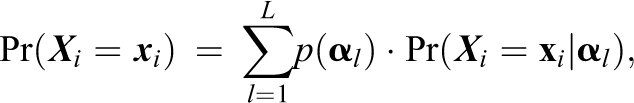
where
A distribution
Thus, let
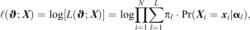
and can be maximized using the EM algorithm as described in de la Torre (2009). The estimation procedure provides the posterior probability for each latent class,
Theory and Estimation of Standard Errors
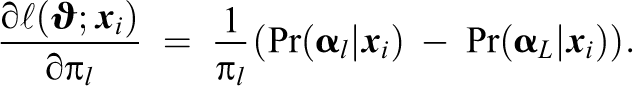
The standard errors of the estimated model parameters
where
Complete and incomplete information matrix
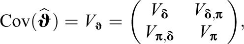
The (asymptotic) covariance matrix of

where

is the score function (i.e., the partial derivatives of the log likelihood with respect to all model parameters).
Similar to the covariance matrix, the information matrix can be divided into four blocks:
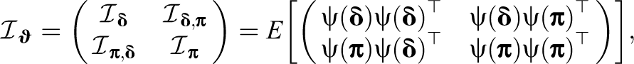
where
In many practical applications (e.g., tests for differential item functioning), researchers are primarily interested in the parameters
The above statement can be derived in a formal way using matrix algebra. Let

with
This means that the standard errors of the estimated parameters
Estimating the information matrix and standard errors
Computing the (expected) information matrix by evaluating the expected value at the ML estimate is infeasible for large assessments. The expectation must be taken over the support of the random response vector
Thus, the information matrix is often estimated by the empirical counterpart of Equation 1, given by
also known as the “outer product of gradients” (OPG) estimator, where
Another estimator follows from the fact that under the true parameter values and standard regularity conditions, the information matrix (as defined in Equation 1) is equivalent to the expected value of the negative Hessian matrix of the log likelihood. Thus, the information matrix may also be estimated via
In practice, however, Equations 3 and 4 are evaluated at the estimated parameter values and, thus, the two estimators differ by
Often Equation 3 is easier to compute, but Equation 4 promises a better finite sample approximation of the information matrix (McLachlan & Krishnan, 2007).
From the above definitions, the standard error for the parameter ϑr (r = 1, …, p + q) can be computed via the inverse of the complete information matrix using

estimated via the outer products of gradients or the Hessian matrix, respectively. Since the differences between the OPG and the Hessian approach turned out to be negligibly small for simple CDMs (i.e., for the deterministic input, noisy “and” gate [DINA] model introduced below, but results are not shown), we will only consider the OPG estimator for the rest of the article.
In the next section, the improvement of the quality of the standard errors using the inverse of the complete information matrix will be illustrated using three specific versions of CDMs. Therefore, we will briefly introduce the G-DINA model framework proposed by de la Torre (2011), which covers other CDMs as special cases. For a comprehensive description of the framework, its relation to other general CDMs and parameter estimation, we refer the reader to the original article.
The G-DINA Model
A comprehensive and very flexible version of a CDM is the G-DINA model (de la Torre, 2011). Due to its general formulation, it includes many other (more restrictive) CDMs as special cases.
For each item in the assessment, the individuals are separated into
Let
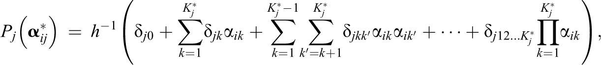
where
The
Other CDMs can be obtained by restricting the parameters in the G-DINA model. An intuitive, simple, and parsimonious CDM is the DINA (Haertel, 1989; Junker & Sijtsma, 2001) model. In the DINA model, the individuals are separated into two latent groups depending on whether they have mastered all the attributes required to solve the item or not. Thus, the DINA model is a completely noncompensatory (or conjunctive) model, which means that having mastered only part of the required attributes does not increase the probability of answering the item correctly. It can be obtained from the G-DINA model by restricting all parameters except
Another CDM that can be obtained from the G-DINA model is the additive CDM (A-CDM). It is slightly more flexible than the DINA model because the conditional response probability can increase (or in some cases decrease) for each attribute that has been mastered. It can be obtained from the G-DINA model by restricting all interaction parameters to zero.
Score contributions for parameters in the G-DINA model
To estimate the information matrix of the model parameters of the G-DINA model via OPG, the contributions of individual i to the score function,
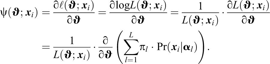
Using formula (A6) from the appendix in de la Torre (2009) for the partial derivative of the conditional likelihood, the score contributions of the parameters of item j can be computed via
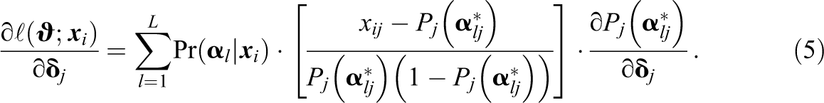
To estimate the score contributions, we plug-in the estimated parameters
For the score contributions of the latent class probabilities, the constraint
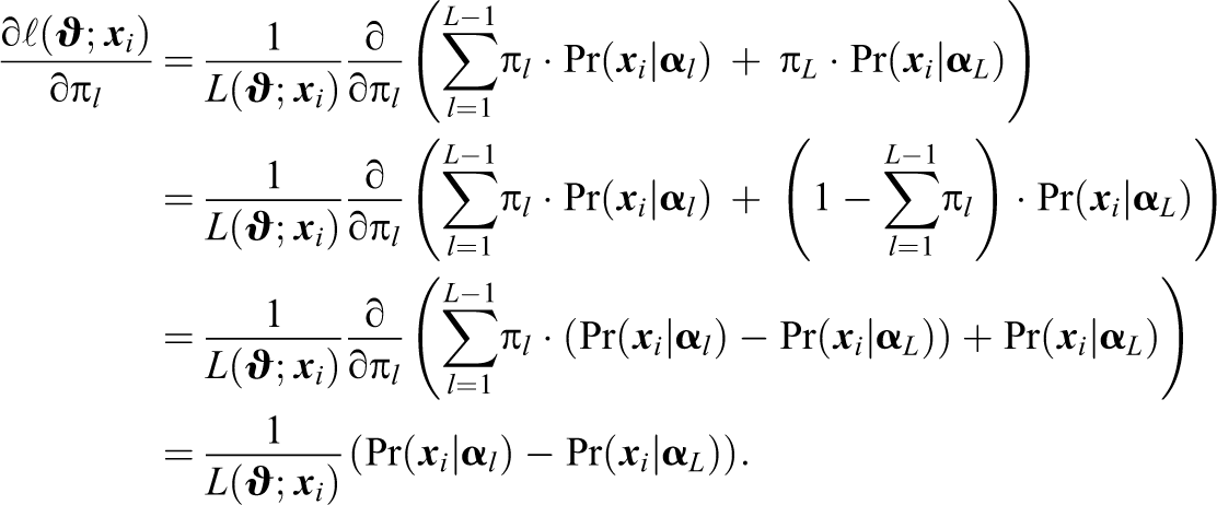
Since the parameters in the last iteration of the EM algorithm are computed from the posterior values
Nonidentifiability of latent classes
In the theory about standard errors of parameters that is presented above, it is assumed that the inverse of the complete information matrix
To avoid problems of identification in practice, it is therefore recommended that, whenever possible, a single-attribute item is included for each of the K attributes when developing new tests for cognitive diagnostic assessment. For researchers who perform a cognitive diagnostic analysis of data from an existing assessment (so-called retrofitting), the inversion problem can be circumvented by pooling latent classes that cannot be separated from each other.
Illustrations
Following the theoretical derivation of the underestimation of the standard errors—resulting from the inversion of the incomplete or the itemwise information matrix—the goal of this section is to illustrate the extent of this underestimation and its effect on confidence intervals for the parameter estimates. In addition, we show for an exemplary real data set how much the standard errors may be underestimated in practice when the wrong methods are used. For both illustrations, the OPG estimator was used to estimate the covariance matrix of the model parameter estimates.
Coverage Study
In the first study, we compare the quality of the standard error estimates based on the complete, the incomplete, and the itemwise information matrix by estimating the coverage probability of the true parameter in a Wald-type confidence interval that uses a normal approximation given by
Four different sample sizes
Transposed Q-Matrix Used in the Simulation Study
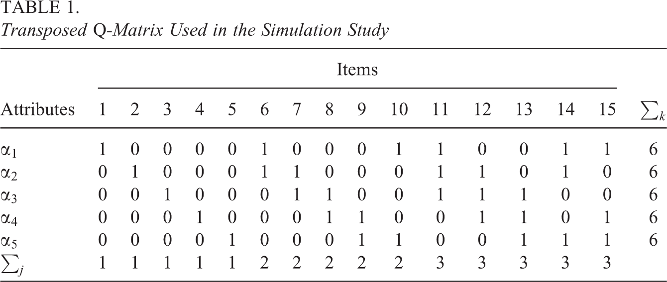
The DINA model and the A-CDM were used to generate response data. For each item, the true value of the baseline parameter
Figures 1 and 2 illustrate the coverage probabilities for the data generated under the DINA model and the A-CDM, respectively. For all sample sizes and models, the coverage probabilities were computed for the
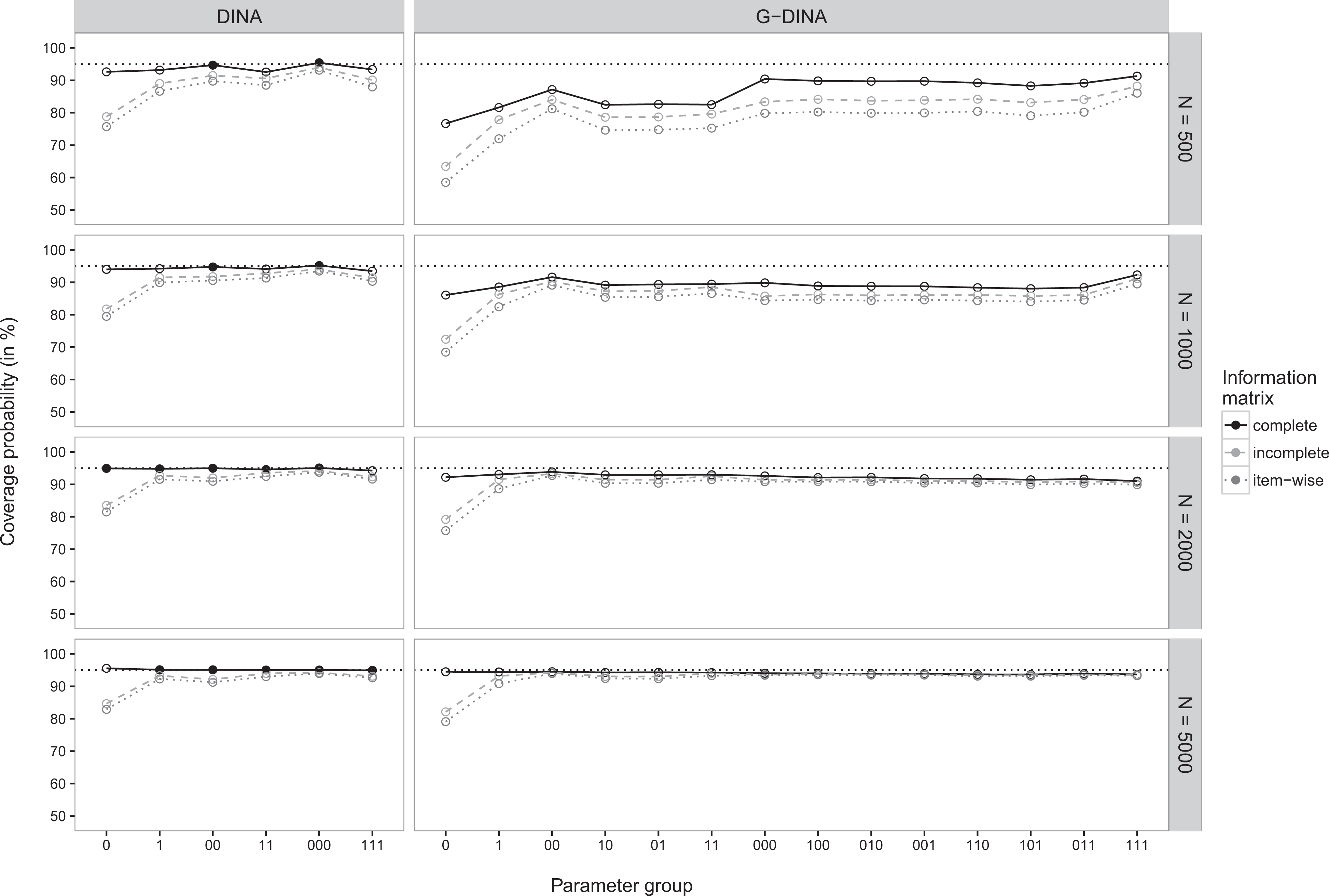
Coverage probabilities of 95% Wald-type confidence intervals for data generated under the deterministic input, noisy “and” gate model are illustrated (on the y-axis) separately for parameters of items that require the same number of attributes (=parameter groups on the x-axis) using three different calculation methods for the standard errors. For ease of readability, values sufficiently close to the nominal coverage probability are depicted as solid circles, all others as empty circles.
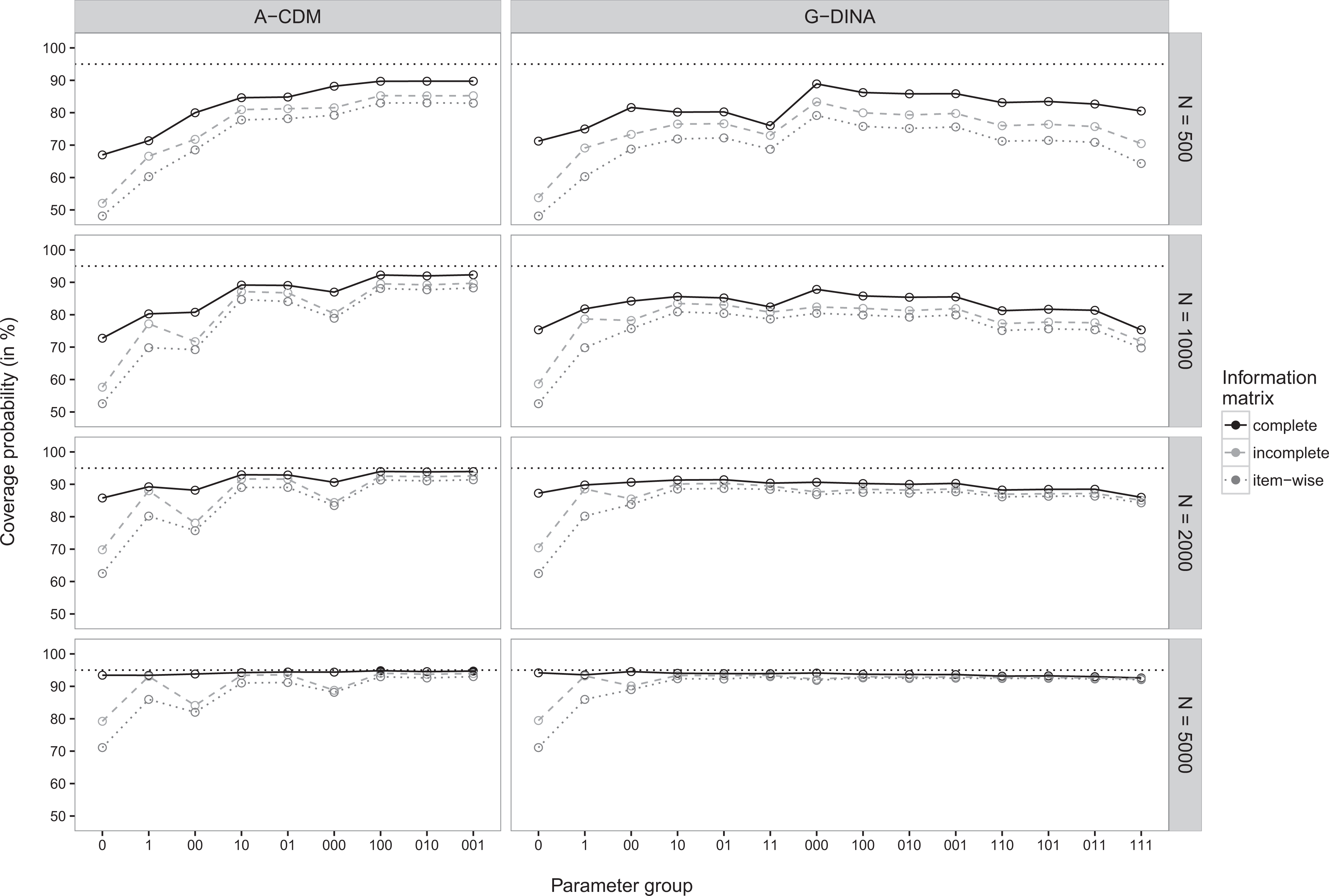
Coverage probabilities of 95% Wald-type confidence intervals for data generated under the additive CDM are illustrated (on the y-axis) separately for parameters of items that require the same number of attributes (=parameter groups on the x-axis) using three different calculation methods for the standard errors. For ease of readability, values sufficiently close to the nominal coverage probability are depicted as solid circles, all others as empty circles.
By definition, the coverage probability of a 95% confidence interval has an expected nominal coverage rate of 95%. However, due to sampling error, the estimated coverage probabilities may randomly deviate from this nominal value. To achieve a high precision of the estimated coverage probabilities, each configuration was repeated 10,000 times. Assuming an exact binomial distribution for the coverage probabilities, the sampling error was equal to
Additionally, Tables 2 through 5 list the exact values of the coverage probabilities and the empirical bias of the standard errors for the smallest (N = 500) and the largest (N = 5,000) sample sizes (the intermediate sample sizes were omitted for brevity but can be requested from the corresponding author) and each parameter group (labeled by η). The average empirical bias corresponds to the average of the empirical biases over all replications that were computed by subtracting the estimated standard errors
Coverage Probabilities of 95% Wald-Type Confidence Intervals and Average Estimated Bias of the Standard Errors for Data Generated Under the DINA Model and Fitted to the DINA Model
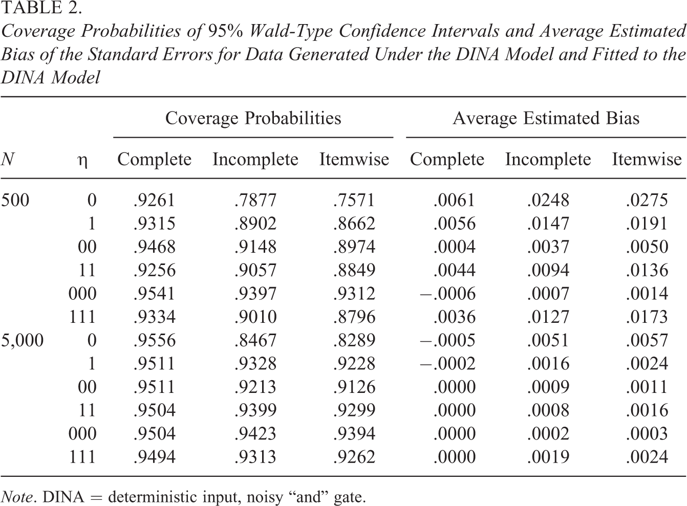
Note. DINA = deterministic input, noisy “and” gate.
Coverage Probabilities of 95% Wald-Type Confidence Intervals and Average Estimated Bias of the Standard Errors for Data Generated Under the DINA Model and Fitted to the Overspecified G-DINA Model
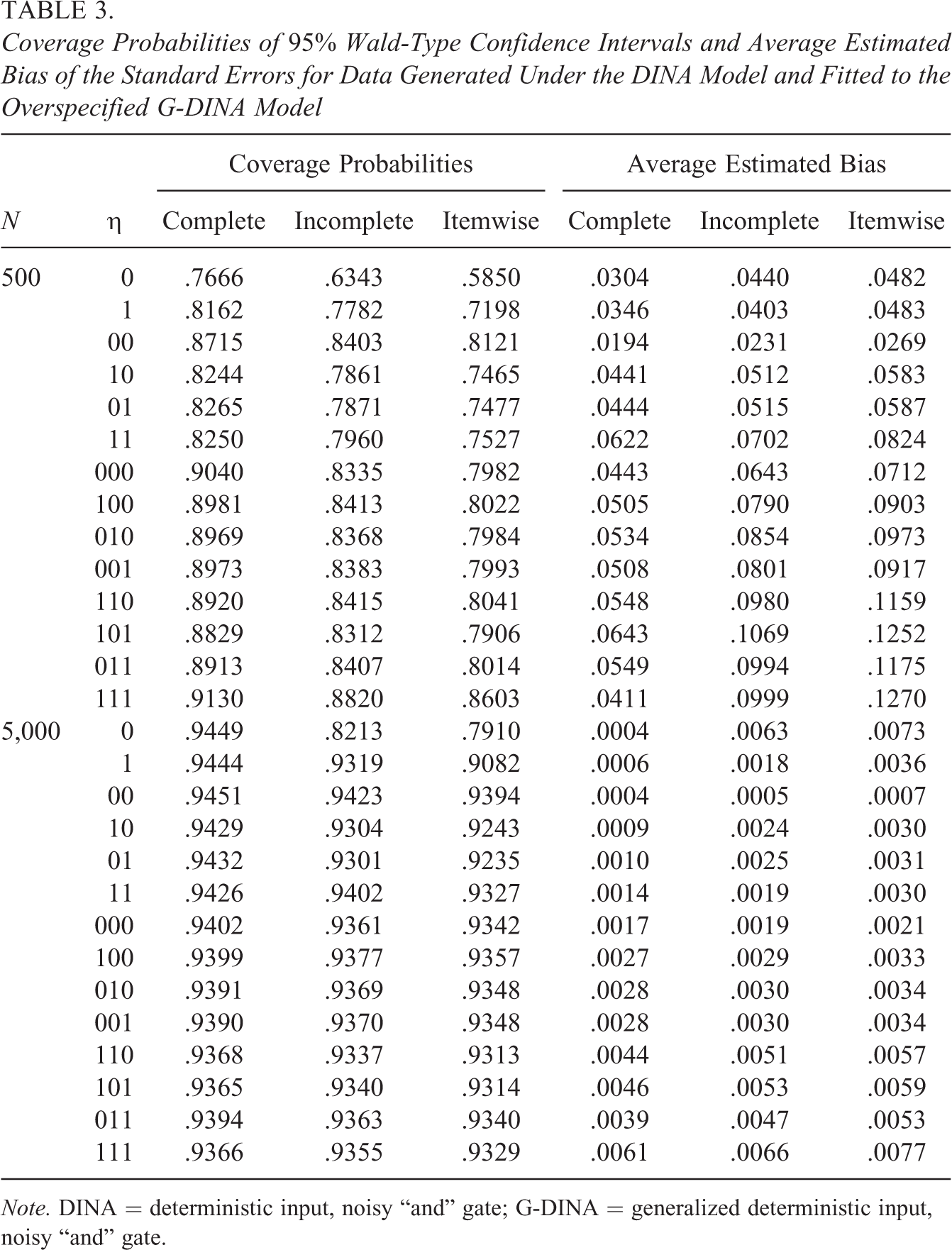
Note. DINA = deterministic input, noisy “and” gate; G-DINA = generalized deterministic input, noisy “and” gate.
Coverage Probabilities of 95% Wald-Type Confidence Intervals and Average Estimated Bias of the Standard Errors for Data Generated Under the A-CDM and Fitted to the A-CDM
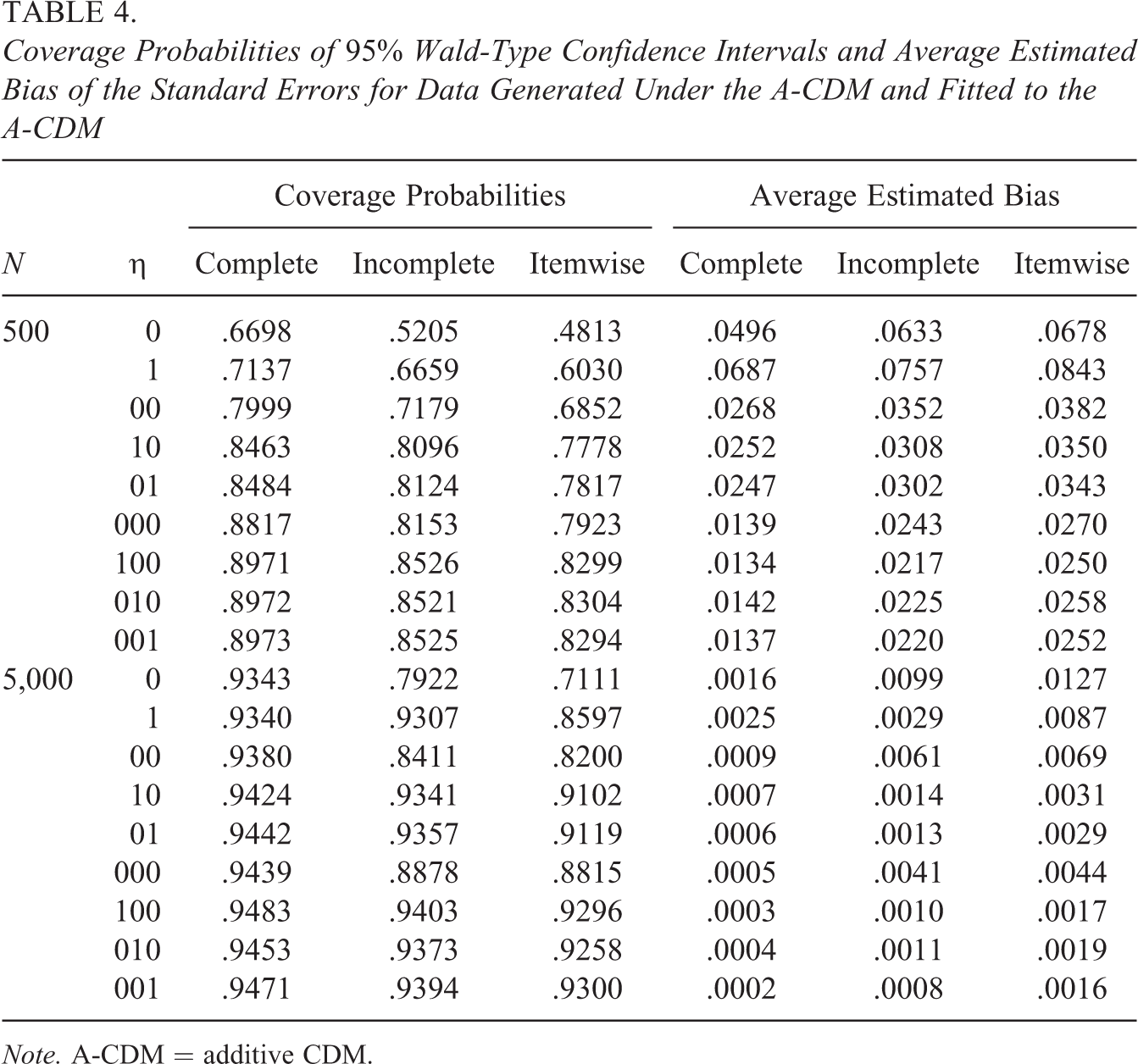
Note. A-CDM = additive CDM.
Figure 1 shows the coverage probabilities for the data generated under the DINA model. When the DINA model was used to analyze the data (see left column in Figure 1 and exact values reported in Table 2), the coverage probabilities for the standard errors based on the complete information matrix (solid line) were reasonably close to the expected coverage rate for small data samples and converged quickly toward the nominal rate with increasing sample size N. The coverage rates for the standard errors based on the incomplete (dashed line) or the itemwise (dotted line) information matrix, however, were systematically smaller than the nominal coverage probability, particularly for the first parameter groups. Even for the largest sample size considered, their coverage probability does not converge toward the nominal rate. This is caused by the structural underestimation of the standard errors discussed earlier. We observed the largest underestimation for the baseline probabilities of single-attribute items (parameter group “0”). For the other parameters, the difference to the correct approach is smaller but still lower than for the correct approach and notably below the nominal rate. A similar pattern can be observed when the G-DINA model was used to analyze the data generated under the DINA model (see right column in Figure 1 and exact values reported in Table 3). However, for smaller sample sizes, the coverage probabilities were generally estimated considerably below the nominal coverage rate of 95%. This artifact may be explained by several circumstances. First, the normal approximation underlying the Wald-type confidence intervals might fail, particularly for the baseline probabilities that are restricted between zero and one. Second, for smaller data sets and more complex models, the conditional response probabilities and the parameters used to specify the attribute distribution are often estimated on the boundary of the parameter space. As mentioned earlier, this causes numerical problems in the calculation of the information matrix. Finally, the ratio between the number of estimated parameters per observation is larger for more general models. Thus, inferior asymptotic convergence has to be reckoned with the G-DINA when compared to the DINA model. Nevertheless, the complete information matrix approach clearly provided more accurate results in all the conditions considered.
Similar and related conclusions can be drawn from the average empirical biases reported in Tables 2 and 3. They were (in absolute terms) always smaller when the complete information matrix instead of the incomplete or the itemwise information matrix approaches were used. Please note that when the correct DINA model was fitted to the simulated data (see values reported in Table 2), and when the standard errors were estimated with the complete information matrix approach, the bias almost completely vanished for the larger sample size, whereas with the two incorrect approaches still had significant biases at the larger sample size. This, however, was not the case when the overspecified G-DINA model was fitted to the data simulated under the DINA model (see values reported in Table 3). The average estimated biases reported for the complete information matrix approach did not coverage zero, although it was always smaller than for the incomplete and the itemwise approaches. Despite this finding, the complete information matrix approach provided the most accurate standard error estimates of all estimation approaches considered in this study.
Figure 2 shows the coverage probabilities for the data generated under the A-CDM (for exact values, see Tables 4 and 5) . For the same reasons as discussed above, the coverage probabilities were estimated below the nominal rate for smaller samples. As the sample size increased, the coverage probabilities computed with the standard errors based on the complete information matrix again approached the nominal rate for the A-CDM and the G-DINA model. The coverage probabilities computed with the standard errors based on the incomplete or the itemwise information matrix, however, were again systematically underestimated. Overall, the complete information matrix approach again provided more accurate results across all conditions considered.
The average empirical biases reported in Tables 4 and 5 were again always smaller with the complete information approach for all parameter groups and sample sizes. However, as discussed above for the data simulated under the DINA model, the bias did not converge toward zero for the larger sample size, when the overspecified G-DINA model was used to estimate the data simulated under the A-CDM (see values reported in Table 5).
Coverage Probabilities of 95% Wald-Type Confidence Intervals and Average Estimated Bias of the Standard Errors for Data Generated Under the Additive CDM and Fitted to the Overspecified G-DINA Model
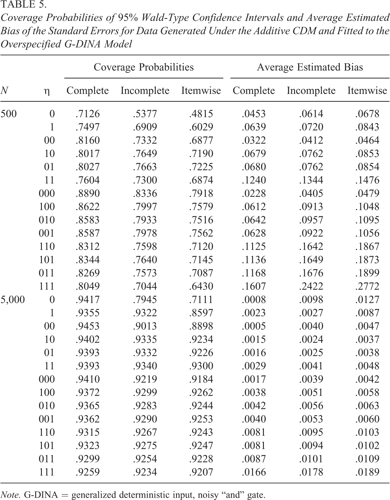
Note. G-DINA = generalized deterministic input, noisy “and” gate.
Empirical Example
To illustrate the practical importance of estimating standard errors via the complete information matrix, data from a real assessment were analyzed using CDMs. The data stem from a learning experiment at the University of Tuebingen in Germany and is available in the R package the classic probability of an event (pb)? the probability of the complement of an event (cp)? the probability of the union of two disjoint events (un)? the probability of two independent events (id)?
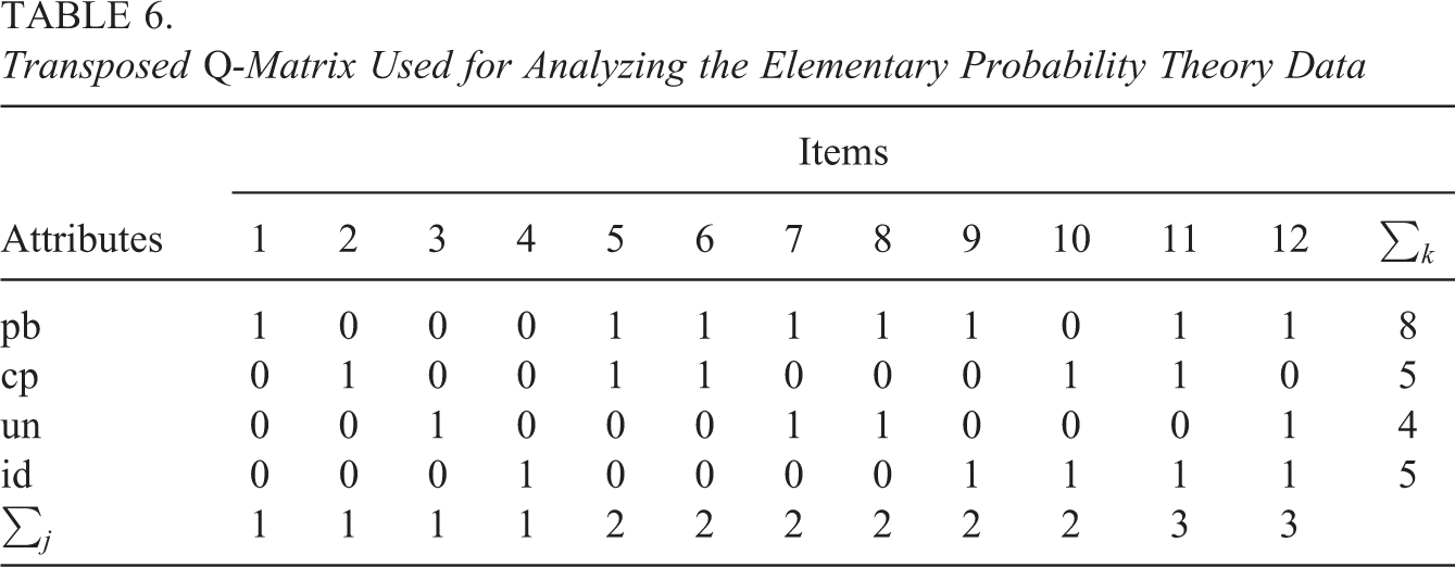
These concepts were combined to form the 12 items. Therefore, the Q-matrix (see Table 6) was defined by the design of the items. The first 4 items required only one attribute, Items 5 through 10 required two attributes, and Items 11 and 12 required three attributes. For this illustration, the responses of 504 participants from the first part of the experiment were analyzed.
Transposed Q-Matrix Used for Analyzing the Elementary Probability Theory Data
The data were fitted using the DINA, the A-CDM, and the G-DINA model with the resulting Bayesian information criterion (BIC) values of 5,200.46 (df = 39), 5,154.58 (df = 49), and 5,241.70 (df = 63), respectively. The results of the A-CDM—which had the lowest BIC value—are illustrated in Table 7. The table summarizes the estimated parameters; the corresponding standard errors based on the complete, the incomplete, and the itemwise information matrix; and the relative change in the standard errors between the correct and the two incorrect approaches (in parentheses).
Estimates and Standard Errors of Parameters for the Elementary Probability Theory Data
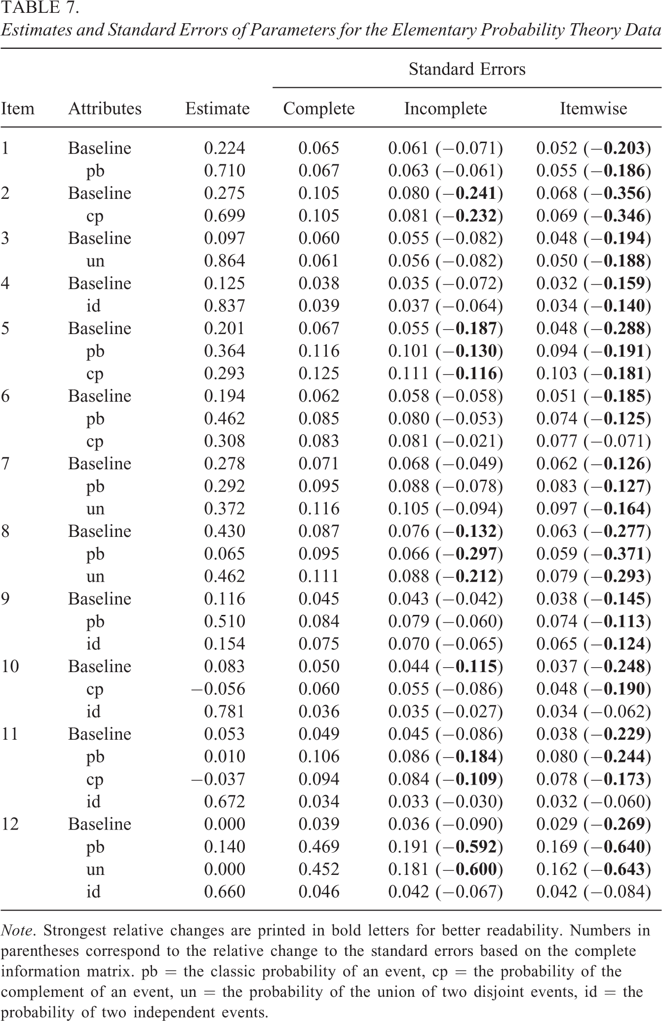
Note. Strongest relative changes are printed in bold letters for better readability. Numbers in parentheses correspond to the relative change to the standard errors based on the complete information matrix. pb = the classic probability of an event, cp = the probability of the complement of an event, un = the probability of the union of two disjoint events, id = the probability of two independent events.
For each item, the first parameter estimate represents the baseline probability (i.e., the probability of correctly answering the item when the attributes required by the item have not been mastered). Thus, large values for this guessing probability are unusual. For Item 8, however, a value of over .4 is reported. A possible explanation is that the item—“What is the probability of obtaining an odd number when throwing a dice?”—was not very difficult, even for individuals without knowledge in basic probability theory. Further parameter estimates represent the amount of increase (or seldom decrease) in probability of answering an item correctly when the corresponding attribute had been mastered. For example, the probability of answering Item 1 increased by .71 when attribute “pb” had been mastered.
The relative change between the standard errors based on the complete and the incomplete information matrix showed substantial differences (highlighted by bold letters in Table 7) for both parameters of the single-attribute Item 2; for some of the parameters of the two-attribute Items 5, 8, and 10; and for some of the parameters of the three-attribute Items 11 and 12. The underestimation of the standard errors based on the itemwise information matrix was even worse. For 30 of the 34 item parameters, the standard error was underestimated.
It should be noted that 10 of the 48 conditional response probabilities and 4 of the 16 parameters of the latent class probabilities were estimated at the boundary of the parameter space (not displayed in Table 7). As mentioned earlier, this can cause numerical problems in computing the information matrix. According to the previous simulation study, where a similar scenario was investigated (see top-left panel in Figure 2 for the same model and a nearly equal sample size), it must be assumed that some of the standard errors reported for these data are generally underestimated. Nevertheless, just like in the simulation study—and as expected from our theoretical considerations—the additional severe underestimation caused by the wrong computation of the information matrix can easily be avoided using the complete information matrix.
Discussion
Standard errors are an important measure to quantify the uncertainty of an estimate. They are required for many different statistical techniques to evaluate model fit or to check model assumptions. It is therefore crucial in practical research to estimate standard errors as precisely as possible. In the commonly used approach for computing standard errors in CDMs, however, the information matrix is based only on those parameters that are used to specify the item response function. The parameters used to specify the joint distribution of the attributes (i.e., latent class distribution) are not incorporated in the computation.
In this article, we have shown that with this approach, the standard errors for the parameters of the item response function are systematically underestimated. We therefore strongly recommend to compute the standard errors based on the complete information matrix, which also includes the parameters used to specify the latent class distribution. In addition to the clear theoretical result, we have illustrated by means of simulations that our approach leads to a higher quality of Wald-type confidence intervals and lower empirical bias. An additional benefit of using the complete instead of the incomplete information matrix is that it also provides the information required to compute standard errors for the parameters used to specify the latent class distribution.
We assume that the incomplete information matrix approaches have only become widely used in the CDM literature because previous authors might have assumed that the off-diagonal elements of the information matrix would have negligible impact under certain conditions. With respect to the itemwise computation of the standard errors, the CDM literature may be partially influenced by the traditional IRT literature, where approaches exist that lead to block diagonal information matrices (e.g., in Thissen & Wainer, 1982), in which case an itemwise computation of the standard errors is possible. However, for CDMs, as we showed analytically and illustrated with examples, the complete information matrix approach clearly generates better standard errors than the incomplete and the itemwise approaches and is computationally well feasible. Similar to our results, Yuan, Cheng, and Patton (2014) showed that the itemwise computation of the standard errors in IRT models also leads to undersized standard errors.
In the simulation study, we did not specifically vary design factors such as the Q-matrix, the true values of the item parameters, or the latent class distribution. Varying these factors might positively or negatively affect the severity of underestimation. In a preliminary study with the DINA model, we found that longer tests and highly discriminating items can alleviate the underestimation. It should be highlighted, however, that the proposed method for estimating the standard errors cannot make the quality of the standard errors worse. In practical situations, however, it is difficult (or even impossible) to control the factors that have a large impact on the underestimation. As such, it is always preferable to compute standard errors using the complete information matrix.
We note that differences between the approaches are expected not only for the standard errors but for the entire covariance matrix of the model parameters (although not generally in the same direction). Thus, many techniques used to investigate a fitted model may be affected. The impact of under- or overestimation of the entire covariance matrix will be multiplied for multivariate methods. It is therefore worth in any circumstances to estimate standard errors (and also the entire covariance matrix) from the complete information matrix. As we did not specifically investigate the impact of misestimating the entire covariance matrix on multivariate techniques, it will be interesting for future research to investigate how much the quality of the covariance matrix can be improved using the complete information matrix in computing it.
The results of the simulation study revealed problems of asymptotic convergence when more complex models were fitted to smaller data sets. This might partially be caused by boundary problems that often occur for smaller data sets. DeCarlo (2011) suggested PM estimation to overcome these problems. Whether PM estimation leads to more accurate parameter and standard error estimates than the traditional ML approach in CDMs was not the scope of this work but something that can be investigated in future research. Moreover, the normal approximation of the ML estimates might be more accurate on the real line under the logit link rather than on the (bounded) probability scale under the identity link. However, this not only concerns the estimation of standard errors but of the model parameters in general. Therefore, this is beyond the scope of this article and is not pursued here. It might be of interest for future research, though, to explore the potential benefits of different link functions. In general, the results from our simulation study suggest that it is recommended to use simpler models whenever possible and appropriate because it may avoid boundary problems or problems with asymptotic convergence.
Finally, in the present article, we assumed that the Q-matrix is known or well specified for an assessment. However, in practice (especially when retrofitting CDMs to existing data), the Q-matrix may be unknown or misspecified, which can affect parameter estimation and classification accuracy (de la Torre, 2008; Rupp & Templin, 2007). To minimize the impact of a misspecified Q-matrix, several methods have been proposed. De la Torre (2008) proposed an iterative procedure to evaluate the correctness of the Q-matrix specification in the context of the DINA model. The approach was extended by de la Torre and Chiu (2016) to apply generally to other CDMs. Other recent approaches include that of Y. Chen, Liu, Xu, and Ying (2015), which estimates the Q-matrix of the DINA model using regularization, whereas Chiu (2013) proposed a nonparametric approach to Q-matrix validation that does not require specifying the exact form of the CDM, only that the underlying process is conjunctive in nature. Future research should examine the extent of the impact of Q-matrix misspecifications on standard error estimation, and whether specific steps can be taken to minimize such an impact.
Computational Details
The estimation routines used in this study were written in the free and open-source software R (R Core Team, 2016) for statistical computing. Functions to estimate the parameters and the standard errors in the G-DINA model are provided in the form of the add-on package
Footnotes
Appendix
Declaration of Conflicting Interests
The author(s) declared no potential conflicts of interest with respect to the research, authorship, and/or publication of this article.
Funding
The author(s) received no financial support for the research, authorship, and/or publication of this article