More Than One Replication Study Is Needed for Unambiguous Tests of Replication

Abstract

The problem of assessing whether experimental results can be replicated is becoming increasingly important in many areas of science. It is often assumed that assessing replication is straightforward: All one needs to do is repeat the study and see whether the results of the original and replication studies agree. This article shows that the statistical test for whether two studies obtain the same effect is smaller than the power of either study to detect an effect in the first place. Thus, unless the original study and the replication study have unusually high power (e.g., power of 98%), a single replication study will not have adequate sensitivity to provide an unambiguous evaluation of replication.

Keywords

educational policy evaluation experimental design meta-analysis program evaluation research methodology validity/reliability

Introduction

The idea that scientific studies can be replicated is fundamental to the rhetoric of the scientific method and is part of the logic supporting the notion that science is self-correcting because replication attempts will identify findings that are incorrect (see, e.g., McNutt, 2014). During the last decade, the replicability of scientific findings has been called into question by empirical analyses in medicine (e.g., Collins & Tabak, 2014; Ioannidis, 2005; Perrin, 2014), psychology (e.g., Open Science Collaborative, 2015), and economics (e.g., Camerer et al., 2016). Scientists themselves appear to be concerned about replicability in many disciplines (e.g., Baker, 2016) including psychology (e.g., Pashler & Harris, 2012). This concern has been echoed in the popular press, with articles in Newsweek, The Economist, and The Atlantic questioning the replicability of scientific work. It seems likely that evidence that the findings of scientific research cannot be replicated may undermine both the credibility of science and enthusiasm for funding scientific research.

Because the concept of replication is so important to science, one might expect that precise definitions of what constitutes a replication, how to design replication studies, and how to analyze their results would be well known in the scientific literature. As Schmidt (2009) puts it,

one would expect there to be a large body of literature on replication providing clear-cut definitions on such matters as “what exactly is a replication experiment?” or “what exactly is a successful replication?” Furthermore, one would expect to find guidelines on how to conduct a replication or maybe some standard operating procedures on this issue.…The opposite is true. (p. 90)

Much of the existing literature on replication focuses on the definition and functions of replication not on the design or analysis of replication studies (see, e.g., Gomez, Juristo, & Vegas, 2010; Lykken, 1968; Sidman, 1960). Schmidt (2009) argues that previous philosophical and psychological literature on replication largely makes a distinction between two types of replication. One is direct replication, which means “Repetition of an experimental procedure” (p. 91). The other is conceptual replication, which means “Repetition of a test of a hypothesis or a result of earlier research work with different methods” (p. 91). Schmidt then goes on to evaluate the types of replication in the social sciences but offers little discussion of the design or analysis of replication studies.

While the analytical question of how to decide whether the findings from a set of studies should be regarded as supporting replication has been debated for many years (see, e.g., Humphreys, 1980), it is hardly settled. For example, the Open Science Collaboration (2015) conducted one replication of each of a set of 100 published studies in psychology. When analyzing the results of their project, they claimed, “There is no single standard for evaluating replication success” and used five different (and in some cases inconsistent) ways of evaluating whether the studies replicated. The analytic methods they used (and their conclusions) were almost immediately challenged (see, e.g., Etz & Vandekerckhove, 2016; Gilbert, King, Pettigrew, & Wilson, 2016; Hartgerink, Wicherts, & van Assen, 2017; van Aert & van Assen, 2017). A replication project in economics similarly stated that “There are different ways of assessing replication, with no universally agreed-upon standard of excellence” and also evaluated replicability in several different ways (Camerer et al., 2016).

It is notable that both of these large, systematic programs of replication studies were carried out without a specific criterion for what replication would mean (a precise definition of replication). Moreover, these projects were not designed using principles that would ensure conclusive results based on any one of the metrics they used. In contrast, agencies that fund clinical trials or large field experiments in education, such as the U.S. National Institutes of Health (NIH) or Institute of Education Sciences (IES), routinely require projects, before they are funded, to provide precise specification of analyses to be done and power calculations to support the claim that the study’s results will be unambiguous. That is, they require a demonstration that the power of the proposed study will be high enough that a failure to reject the null hypothesis could be interpreted as a failure to find an effect of the smallest size that is deemed important. It appears that no such principles were used to justify that analyses in either of these two high-profile research efforts would lead to unambiguous conclusions.

The focus on analysis of replication is important because there are pervasive examples of misinterpretation of replication studies. Suppose Study A finds that a treatment has a statistically significant effect, but Study B does not, this is often called a “failure to replicate” and is one criteria used in the articles described above. Similarly, if studies A and B both find statistically significant (or both find statistically insignificant) effects, this is often called a “replication.” The fact that differences in conclusions from statistical significance tests do not necessarily correspond to differences in study effects but are often interpreted as doing so has been noted for many years (see, e.g., Gelman & Stern, 2006; Hedges & Olkin, 1985, chapter 1; Humphreys, 1980). It is also true that inference about the overall results of two or more studies based on the outcomes of statistical significance tests in each one (i.e., deciding that the overall effect is nonzero based on the proportion of studies that find a statistically significant result) has remarkably poor properties as an inference procedure (Hedges & Olkin, 1980).

Despite the lack of apparent consensus on how to statistically evaluate replication, systematic replication efforts such as those by the Open Science Collaboration suggest that scientists generally believe that evaluation of whether a study’s results replicate is a straightforward process: Simply repeat the experiment (with the same or perhaps an even larger sample size than the original), compare the results of the two studies, and see if they are “the same.” However, precisely what is meant by the same, how to assess that definition, and what data are needed to do so remain somewhat unsettled matters. Note that the problem of planning a data collection to evaluate whether the results of a study replicate is fundamentally a research design problem. It specifies a design in the form of an ensemble of studies (in this case, two studies, the original and the replication study) and specifies data collection procedures (the same as the original study with at least the same sample size) for each study in the ensemble.

This article addresses the question of whether an ensemble of two studies (the original study and a single replication study) can ever be sufficient to obtain conclusive evidence about whether a result has or has not been replicated. Our focus is on the types of direct replications conducted so far in the social sciences, where the goal is to obtain results that might be considered the same across replication studies. We review the importance of adequately sensitive research designs for statistical analyses, and their implications in the context of replication. Using meta-analysis as framework, we clarify subjective notions about replication (i.e., getting the same results) and describe relevant statistical analyses. We then demonstrate that the statistical uncertainty inherent in comparisons between the results of two studies is larger than that of the result of either study alone. Thus, a single replication study cannot usually lead to unambiguous statistical conclusions about replication. We conclude that serious statistical research on the design of ensembles of replication studies is needed to support scientific efforts to evaluate replication.

Research Design and Statistical Analysis

Research design should be informed by some evaluation of whether the design is sufficiently sensitive so that the findings from it will be unambiguous. Statistical analyses are unambiguous only when they are sufficiently sensitive. The two most frequently used modes of statistical analysis are hypothesis testing (statistical significance testing) and estimation of effects or effect sizes. These two modes of analysis are closely related, and each has established concepts of sensitivity.

For hypothesis testing, sensitivity can be characterized by the statistical power of the test. Researchers posit well-formed null hypotheses, and the analysis determines whether the data are sufficient to reject that hypothesis. Typically, in the context of a single experiment, the null hypothesis is of no (or a negligible) effect. Rejection of the null hypothesis is conclusive because the test is designed, so that it will have only a small chance of rejecting the null hypothesis if it is true. That small chance is called the significance level and is determined a priori by the investigator.

On the other hand, failure to reject the null hypothesis is more ambiguous, and this is where the sensitivity of the test becomes important for interpretation. Statistical power provides a measure of that ambiguity. It is the probability that the statistical analysis would have detected the smallest real effect that is deemed nonnegligible (the smallest effect “worth detecting”). This probability depends on the design and analysis of the investigation, the level of statistical significance, and the definition of the largest effect that is nonnegligible (worth detecting). The bigger the smallest effect worth detecting, the higher the statistical power.

When the statistical analysis has low power, failure to reject the null hypothesis is inherently ambiguous: It could mean that the real effect is negligible (or null), or there could be a nonnegligible real effect that goes undetected due to low sensitivity. Designing experiments so that they will have high statistical power reduces the ambiguity of interpreting nonstatistically significant findings. This is why agencies that fund large-scale clinical trials (e.g., NIH or IES) require power analyses in proposals for funding of such trials. While there is currently a strong scientific consensus that significance levels should be set to 5%, there is less of a consensus on how high statistical power should be, but the idea that 80% power is adequate has been broadly embraced in the social sciences (Cohen, 1977).

When estimation is used as the analytic technique, sensitivity can be characterized by the standard error (SE) or the width of the confidence interval for the estimated effect. There are no firmly established standards for desirable precision or confidence interval width, but there is a general understanding that precision should be high and confidence intervals should be narrow relative to the quantity being estimated.

The virtues of research designs that have high sensitivity have been well known for some time. However, research designs that have high power or high precision are generally costly because such sensitivity is usually obtained by using large sample sizes. Not surprisingly, there is ample evidence that research studies in medicine and the social sciences are often less sensitive than would be desirable (see, e.g., Dumas-Mallet, Button, Boraud, Gonon, & Munafò, 2017; Vankov, Bowers, & Munafò, 2014).

It would seem that sufficiently sensitive designs would be of particular interest for studying replication. The replicability of findings is central to the idea that they are scientific, and so evaluations of replicability should be conclusive as part of good science. In addition, conducting replications will require resources that may otherwise have been devoted to exploring new questions. And while resolving which (novel research vs. replication) should be a priority cannot be solved by statistics alone, at the very least, considerations about design should be used to ensure that resources are not devoted to replication research that nets ambiguous results.

The Statistical Analysis of Effect Heterogeneity in Meta-Analysis

The most relevant statistical literature for considering the analysis of replications is that of meta-analysis, which offers methods for statistically combining results across studies (see, e.g., Cooper, Hedges, & Valentine, 2009; Hedges & Olkin, 1985). However, meta-analysis has been more concerned with summarizing effect sizes from a set of studies than evaluating whether studies replicate according to stated criteria. Moreover, meta-analysis is mostly concerned with problems of summarizing existing studies, not with the problem of designing ensembles of studies to evaluate replicability. Yet, because meta-analysis is a widely accepted method of combining evidence in many areas of science, our approach is in the spirit of meta-analysis and uses meta-analytic methods.

In the meta-analytic framework, a study’s results can be summarized by an effect parameter θ, which is the result the study would have obtained if there were no estimation errors due to the sampling of experimental units (e.g., if the sample size were infinite). The effect size might be a treatment–control mean difference, a standardized mean difference, a correlation coefficient, log-odds ratio, or any standard meta-analytic effect size. While the true result of the study (unperturbed by estimation error) is represented by the effect size parameter θ, we do not observe this parameter in studies with finite sample size. Instead, we observe an estimate T of θ. For discussions of a variety of effect sizes that are often used in education and the social sciences and their properties, see, for example, chapters 12 and 13 of Cooper, Hedges, and Valentine (2009).

Suppose that two studies are potential replicates of one another. Let θ₁ and θ₂ be the effect size parameters from the studies and let T₁ and T₂ be the effect size estimates with known estimation error variances v₁ and v₂. Assume that the effect size estimates are approximately normally distributed so that

T_{i} \sim N (θ_{i}, v_{i}) .

We argue that replication can be described in terms of the effect parameters since they are the scientific quantities of interest in the analysis of any single study. If the studies successfully replicate, then θ₁ and θ₂ should be similar, and if they do not successfully replicate, then θ₁ and θ₂ must be different. Thus, given the two modes of statistical analysis, evaluating whether the two studies successfully replicate can be done by conducting a hypothesis test about the difference between θ₁ and θ₂ or by estimating the magnitude of that difference. If these analyses are not sensitive, then analyses about whether a scientific finding is replicated will be ambiguous.

A primary statistical tool used in meta-analysis to assess differences between effect parameters is the Q-statistic, and it forms the basis of the analyses described in this article. The Q-test in meta-analysis is widely used because it is the likelihood ratio test for heterogeneity under the model described above and so has certain optimal properties. When there are only two studies, the Q-statistic is given by

Q = {(T_{1} - T_{2})}^{2} / (v_{1} + v_{2}) .

When $θ_{1} = θ_{2}$ , Q has a χ² distribution with one degree of freedom. Note that when there are only two studies, the Q-statistic is just the square of the difference between T₁ and T₂ divided by the SE of the difference (the Wald statistic), so it is equivalent to the two-sided version of that test.

When $θ_{1} \neq θ_{2}$ , the distribution of Q depends on how we conceive of the effect parameters (Hedges & Pigott, 2001). Are they the entire population of parameters of interest, or might we want to make inferences about unobserved (potentially future) studies? The answer to this question has implications for both the scope of inference and the properties of the analysis we might do. In general, the way we frame the question of replication determines the conclusions we can draw and the analyses that support them. Below, we describe theoretical considerations and their implications for an analysis of replication.

Theoretical Considerations in Framing an Analysis of Replication

Do the Observed Studies Comprise the Population or a Sample?

The studies available can be considered in either of two different ways: fixed or random. This determines not only the scope of inference but also the way in which we might characterize differences between studies and the properties of the relevant analyses.

If the studies constitute the entire population of studies relevant to assessing replication, then inferences about replication are inferences about the effect parameters in the studies actually observed. This is consistent with the fixed effects framework in meta-analysis (see, e.g., Hedges & Vevea, 1998). One might say that conclusions about replication in the fixed-studies framework are conclusions about how well the observed studies agree. Statistically, this means that we can define replication directly in terms of the difference between $θ_{1}$ and $θ_{2}$ . Moreover, when we treat the studies as fixed, the sampling distribution of Q depends on the magnitude of (θ₁ − θ₂)² through the noncentrality parameter $λ = {(θ_{1} - θ_{2})}^{2} / (v_{1} + v_{2})$ (see below).

If the studies are considered random, then the studies observed are a sample from a hypothetical population or universe of studies, and their effect parameters are a sample from a hypothetical universe of effect parameters. Inferences about replication are inferences about the universe of effect parameters from which the sample was taken. Thus, the observed studies and their effect parameters are of interest only in that they provide information about these hypothetical universes of studies and their effects. This is consistent with the random effects framework in meta-analysis (see, e.g., Hedges & Vevea, 1998). One might say that conclusions about replication in the random-studies framework are conclusions about how well findings might agree in a universe of studies, where that universe is one which might have yielded the observed studies as a random sample.

In statistical terms, the random-studies framework defines replication in terms of how similar θ _i drawn from the same distribution might be. We can characterize this similarity in terms of the variance of this distribution, τ²; a distribution with a small variance τ² would produce θ _i that are similar. It turns out that the sampling distribution of Q under the random effects model depends on the magnitude of τ².

The difference between these two frameworks may seem trivial; however, there are two important differences. The first is that they answer slightly different questions. The fixed effects model addresses agreement between only the observed studies, while the random effects approach pertains also to an entire population of studies including studies not observed. This is why we need different parameters (λ and τ²) to describe replication depending on the model. Second, when there is not perfect agreement in effect parameters across studies, the Q-statistic has a somewhat different sampling distribution when studies are considered fixed than when they are considered random. This has implications for statistical power and constructing tests for approximate replication (see the following section).

In general, it may seem odd to conduct a random effects analysis on only two studies. We present random-studies analysis methods here not to advocate their use, but rather to describe important issues in analyzing replication studies, as well as to illustrate the types of considerations required to design them.

The Definition of Replication: Exact Replication or Approximate Replication?

To conduct a statistical analysis of replication, it must be defined precisely. One possible definition (which is akin to the null hypothesis of the Q-test in meta-analysis) is exact replication: All studies have exactly the same effect parameter. In the fixed effects model, this would correspond to λ = 0, and in the random effects model, this would imply that τ² = 0. This is logically appealing, but it may be too strict to be useful in scientific practice. Even in physics, there is awareness that even the most careful experiments measuring the same phenomenon exhibit some heterogeneity of results (see, e.g., Hedges, 1987; Olive et al., 2014; Rosenfeld, 1975). Therefore, one might argue that some variation in effects across attempted replication studies might be expected. Small differences in the magnitude of effects may not change the interpretation of a finding, and hence, effect parameters that are not identical may still reflect successful replications.

Thus, replication might be defined as a situation in which effects are “almost the same” across studies, such that almost the same is defined precisely. We regard the specific operationalization of almost the same as a matter of scientific judgment that might well differ across fields. We can define approximate replication in terms of the parameters λ and τ² by choosing values that correspond to negligibly small differences in effect parameters. We offer conventions used in three scientific areas to show how one might quantify this notion.

To illustrate how almost the same might be defined, consider three conventions that have arisen in different sciences for identifying a negligible value of τ² (or λ). In high-energy physics, the Particle Data Group (which has been compiling meta-analyses of high energy physics experiments for over 50 years) concludes that (when there are a total of two studies) a value of Q ≤ 1.25 corresponds to negligible heterogeneity (see Olive et al., 2014). Because the expected value of Q under the studies-fixed model is 1 + λ and 1 + τ²/v under the studies-random model, this implies that λ = 1/4 would be a negligible value of λ and that τ²/v = 1/4 would be a negligible value of τ²/v. In personnel psychology, Hunter and Schmidt (1990) proposed that when the estimation error variance v is at least 75% as large as the total variance of the effect size estimates (v + τ²), then the variance of the effect size parameters τ² could be considered negligible. This implies that values of λ = 1/3 and τ²/v = 1/3 correspond to negligible amounts of heterogeneity in effect size parameters. In medicine, a value of I² = 100% × τ²/(v + τ²) of 40% or less is considered to be “not important” (see section 9.5.2 of Higgins & Green, 2008). This implies that λ = 2/3 and τ²/v = 2/3 would be negligible amounts of heterogeneity. We do not advocate any of these values but merely use them for illustration.

Publication Selection

An important assumption in the results of this article is that Study 1 has already been conducted and (presumably) published. This assumption fixes v₁ and poses the question of designing a replication study in terms of the sample size of Study 2 (and hence v₂). However, there is considerable evidence that published studies often experience selection that favors the publication of those that obtain statistically significant results (publication selection; see, e.g., Dickersin, 2005 and the references cited therein). Such publication selection leads to bias in the observed effect size T₁ that can be quite large, as much as 250% in extreme cases (see Hedges, 1984).

The arguments in this article are structured in terms of the effect size parameter θ₁ in the original study, not the observed effect size estimate T₁. But if T₁ is a biased estimate of θ₁, then it would make sense to adjust for that bias in analyses of replication, and there are several ways to do so. Hedges (1984) provides a maximum likelihood estimator for the effect size that models the selection process explicitly, and several variants of the method have been proposed (McShane, Böckenholt, & Hansen, 2016; Rothstein, Sutton, & Borenstein, 2005). These types of corrections result in a “new” estimate $T_{1}^{*}$ that has variance $v_{1}^{*}$ . Since these methods typically require estimation of additional parameters associated with selection, the corrected estimates tend to have a greater variance, so that $v_{1}^{*} > v_{1}$ . Moreover, adjustments that rely on maximum likelihood methods, such as Hedges (1984), will result in effect estimates that are asymptotically normal. Thus, the analysis methods described in this article can proceed with T₁ and v₁ if there is no publication bias, or with $T_{1}^{*}$ and $v_{1}^{*}$ if there is.

Later in this article, we show that the sensitivity of analyses of replication depends on θ₁ and v₁, and sensitivity tends to improve with more precise estimates of effects (i.e., with smaller v₁). Since publication bias corrections increase the estimation error variance $(v_{1}^{*} > v_{1})$ , analyses that adjust for publication bias are likely to be less sensitive than analyses of studies not subject to publication selection.

Hypothesis Tests and the Burden of Proof

In addition to the considerations above (i.e., studies are fixed or random; replication is exact or approximate; publication bias present in Study 1 or not), hypothesis tests depend on one additional factor: where the burden of proof is placed. If the burden of proof is on nonreplication, then the null hypothesis is that the studies (exactly or approximately) replicate. Rejecting this null hypothesis would mean that we conclude that the studies failed to replicate. Note that this test will be conclusive about failures to replicate, but unless the test has high power, it will be inconclusive about whether studies replicate.

However, if the goal of conducting a replication is to determine that study results are similar, then this is the wrong inferential structure. Instead, the burden of proof should be on replication rather than nonreplication. In this setup, the null hypothesis is that the studies failed to replicate (i.e., λ or τ² are at large), and rejecting the null hypothesis would mean that we conclude that the studies replicate (i.e., λ or τ² are small or null).

Given this additional consideration, Hedges and Schauer (2018) show that there are six different hypothesis tests about replication. These are discussed below in the context of designs with k = 2 studies.

Analyses of Replication and Their Properties

So far, we have outlined a meta-analytic approach to the analysis of replications. The sections that follow detail these analyses in the context when only two studies are conducted (an original and one replicate), as in some of the more high-profile empirical evaluations of replication. We explore the properties of these analyses for fixed-studies and random-studies hypothesis tests, as well as with estimation of differences between effects. In particular, we demonstrate that in many practical situations, the sensitivity of these analyses cannot support unambiguous conclusions for only two studies.

Fixed Effects Hypothesis Tests for Exact Replication

We can test the null hypothesis of exact replication (H₀: θ₁ = θ₂) using the standard Q-test in meta-analysis. Recall that when the effect parameters are identical (so that the studies replicate exactly), Q has a χ² distribution with one degree of freedom. So to conduct an α-level test, we compute Q as in Equation 1 and compare it to the critical value

c_{(1 - α)} = F^{- 1} (1 - α | 0),

where F(x | λ) is the cumulative distribution function of the noncentral χ² distribution with one degree of freedom and noncentrality parameter λ, and c_(1–α) is the level 100(1 − α) percent point of the central χ² distribution (e.g., for α = 0.05, c_(1–α) = 3.84). If Q > c_(1–α), we reject the null hypothesis and conclude that the studies do not replicate.

When studies are conceived as fixed, but when $θ_{1} \neq θ_{2}$ , then Q has the noncentral χ² distribution with one degree of freedom and noncentrality parameter (see Hedges & Pigott, 2001), which is given by

λ = {(θ_{1} - θ_{2})}^{2} / (v_{1} + v_{2}) .

The statistical power of the studies-fixed test for replication is

1 - F [c_{(1 - α)} | {(θ_{1} - θ_{2})}^{2} / (v_{1} + v_{2})],

where F(x | λ) and c_(1–α) are as in Equation 2. Note that in this fixed-studies model the sampling distribution (and therefore the statistical properties) of Q is determined entirely by λ.

Designing a replication study for a sufficiently powerful analysis requires consideration of λ; larger values of λ mean greater power. If the original study has already been conducted, v₁ is fixed. The design decision, then, is how small to make v₂ (which often corresponds to how large to make the sample size of Study 2). We can make v₂ as small as we like by making the sample size of the replication study larger. However, as v₂ tends to be 0, λ tends to be ${(θ_{1} - θ_{2})}^{2} / v_{1}$ , so the maximum power will be

1 - F (c_{(1 - α)} | {(θ_{1} - θ_{2})}^{2} / v_{1}),

where F(x | λ) and c_(1–α) are as in Equation 2. Because there is a limit how large we can make λ and because statistical power is determined by λ, there is a limit to how high the statistical power may be, even if we have an indefinitely large replication study.

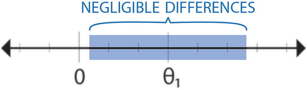
To compute the power of the test for replication, we must decide the smallest nonnegligible value of $| θ_{1} - θ_{2} |$ and the λ value corresponding to this difference: the smallest nonnegligible λ. This is equivalent to specifying a (symmetric) range of θ values above and below $θ_{1}$ which would constitute a “negligible” difference between the results of the two studies. The larger this range of negligible difference, the larger the smallest value of $| θ_{1} - θ_{2} |$ (and λ) worth detecting, and thus the higher the statistical power to detect that difference.

What is the largest this range could be? We would argue that the largest difference that might be considered negligible is one in which both θ₁ and θ₂ have the same sign (there is no qualitative disagreement between effects in Study 1 and Study 2). For example, if Study 1 found a positive effect $(θ_{1} > 0)$ , then θ₂ must also be positive. It follows that when $0 < θ_{2} < θ_{1}$ , it must be true that $θ_{1} - θ_{2} < θ_{1}$ . Thus, the largest λ value that corresponds to a qualitative replication (call it λ _R ) must be less than $θ_{1}^{2} / (v_{1} + v_{2})$ .

A test of the null hypothesis that $θ_{1} = 0$ in Study 1 uses the test statistic $T_{1}^{2} / v_{1}$ , which has the central χ² distribution if $θ_{1} = 0$ and the noncentral χ² distribution if $θ_{1} \neq 0$ . The power of the test is determined by the (noncentrality) parameter $λ_{1} = θ_{1}^{2} / v_{1}$ . Comparing λ₁ to λ _R , we see that

λ_{R} < θ_{1}^{2} / (v_{1} + v_{2}) < θ_{1}^{2} / v_{1} = λ_{1} .

Thus, the maximum possible power of the test for replication is smaller than the power of the original study’s (Study 1) test of the null hypothesis of no effect. However, the maximum possible power may be much lower in theory and almost certainly will be lower in practice for two reasons.

First, power will be lower if we care about smaller differences between study effects rather than just disagreement in sign. If the magnitude of the difference between effects is important, a $θ_{2}$ value that is substantially smaller than $θ_{1}$ , but still positive, might not be considered a replication. In that case, the largest λ _R corresponding to a replication can be substantially less than λ₁. For example, suppose that a reduction in effect of 50% was considered the largest nonnegligible difference between $θ_{1}$ and $θ_{2}$ . In that case λ _R = λ₁/4 and if Study 1 had 80% power to detect $θ_{1}$ (which occurs if $λ_{1}$ = 7.85), then the maximum theoretical power of the test for exact replication would be only 29%. Note that λ_R = 7.85/4 is nearly 3 times the largest value of negligible heterogeneity discussed in the previous section, so in comparison this would be a very loose definition of replication.

A second reason that the power of replication tests must be lower than the theoretical limits above is that the theoretical limits require perfect precision in the replication study (i.e., v₂ = 0 or an infinite sample size). If Study 2 has the same sample size as Study 1, so that, for example, v₁ = v₂, then the largest possible noncentrality parameter of the replication study becomes $θ_{1}^{2} / 2 v_{1} = λ_{1} / 2$ . In this case, if Study 1 had power of 80%, the power of the test for exact replication would be 51%. Even if Study 1 had power of 90%, that of the replication test would be only 63%. Study 1 would have to have a power of 98% for the replication test to have 80% power, which is unusual in many medical or social science contexts.

Additionally, if the analysis corrects T₁ for publication bias, then the procedures above involve the corrected estimate $T_{1}^{*}$ and its variance $v_{1}^{*}$ instead of T₁ and v₁. However, the power of the test still depends on the noncentrality parameter λ, which is a function of the estimation error variance of the first study (v₁ or $v_{1}^{*}$ ). Let $λ^{*}$ be the noncentrality parameter after adjusting for publication bias, and λ be the noncentraily parameter with no adjustment. Note that $λ = {(θ_{1} - θ_{2})}^{2} / (v_{1} + v_{2}) > {(θ_{1} - θ_{2})}^{2} / (v_{1}^{*} + v_{2}) = λ^{*}$ so that the noncentrality parameter after adjustment is smaller than the noncentrality parameter without adjustment. This means that the test for exact replication that corrects for publication bias in Study 1 will be even less powerful than the test when no correction for publication selection is needed.

The greatest theoretical power we may hope to achieve in a test of exact replication is the same as the power of Study 1 to detect a nonzero effect as small as $θ_{1}$ . In practice, the power of the test for replication will be smaller and can be much smaller. Therefore, it may be impossible to design a single replication study to ensure that the analyses of replication are sufficiently sensitive to be conclusive; this is especially true if we consider small differences between study effects to be meaningful.

Fixed Effects Test for Approximate Replication

The test for approximate replication requires the specification of the largest difference between the effect in the original study $(θ_{1})$ and that in the replication $(θ_{2})$ that still qualifies as a replication. Call this difference δ₀, so that the largest value of the noncentrality parameter that corresponds to replication is

λ_{0} = δ_{0}^{2} / (v_{1} + v_{2}),

and the null hypothesis of approximate replication is not that λ = 0 (as in exact replication) but

H_{0} : λ \leq λ_{0} .

To test this hypothesis at significance level α using the Q-statistic, the reference distribution is that of Q when λ = λ₀, so that the test rejects the null hypothesis of approximate replication when Q exceeds the 100(1 − α) percentile of the noncentral χ² distribution with one degree of freedom and noncentrality parameter λ₀. Call this critical value c_(1–α)(λ₀) to emphasize that it is a function of both α and λ₀. When λ > 0, the noncentral χ² distribution is stochastically larger (shifted to the right) compared to the central χ² distribution, so that when λ₀ > 0, c_(1–α)(λ₀) > c_(1–α)(0) = c_(1–α). For example, while c_(1–0.05) = c_(1–0.05)(0) = 3.84, c_(1–0.05)(1/4) = 4.76, c_(1–0.05)(1/3) = 5.03, and c_(1–0.05)(2/3) = 6.06.

The statistical power of the level α studies-fixed test for approximate replication with negligible heterogeneity λ₀ is,

1 - F [c_{(1 - α)} (λ_{0}) | {(θ_{1} - θ_{2})}^{2} / (v_{1} + v_{2})],

where F(x | λ) is the cumulative distribution function of the noncentral χ² distribution with one degree of freedom and noncentrality parameter λ. Here, the noncentrality parameter $λ = {(θ_{1} - θ_{2})}^{2} / (v_{1} + v_{2})$ is the actual heterogeneity expected; it serves the same function as the putative effect size in more conventional power analyses. Comparing the expression for statistical power of the test for approximate replication in Equation 6 with that for the test of exact replication in Equation 4, we note that the only difference is the critical value used. Because tests for approximate replication use the same test statistic, but larger critical values than the test for exact replication, the statistical power of tests for approximate replication to detect the same amount of real heterogeneity is lower than that of the test for exact replication. Therefore, if tests for exact replication based on a single study are insufficiently powerful, tests for approximate replication (including ones that correct for publication bias) will be even less powerful.

Fixed Effects Tests for Nonreplication

The tests above will be conclusive about failures to replicate, but not about replication. If we wish to make conclusive statements about studies successfully replicating, then the burden of proof should be on replication. In that case, the null hypothesis would be that the studies do not replicate, and concluding otherwise would require convincing evidence that they do.

Forming a null hypothesis that the studies fail to replicate involves some consideration of the smallest difference between θ₁ and θ₂ that might be considered nonnegligible. This can be operationalized by the following null hypothesis:

H_{0} : λ \geq λ_{0}

Note that this is the opposite of the null hypothesis of the test for approximate replication in the previous section. Here, the true difference between studies is characterized by λ = δ²/(v₁ + v₂) such that δ = θ₁ − θ₂. In this test of nonreplication, the null hypothesis is that this value λ is at least as large as a difference characterized by $λ_{0} = δ_{0} / (v_{1} + v_{2})$ , where $δ_{0}$ corresponds to the smallest nonnegligible difference between studies (i.e., the smallest value of δ that corresponds with nonreplication).

Hedges and Schauer (2018) show that to test this null hypothesis with level α, one computes Q as in Equation 1 and rejects the null hypothesis if it is less than the critical value c_α(λ₀), the 100α percent point of the distribution of Q when λ = λ₀:

c_{α} (λ_{0}) = F^{- 1} (α | λ_{0}),

where F is the χ² distribution function as in Equation 2.

The power of this test to detect λ < λ₀ is given by

F [F^{- 1} (α | λ_{0}) | λ] .

The power increases as λ decreases and is greatest when the studies replicate exactly so that λ = 0. The power is also an increasing function of λ₀, which means that it is higher as we test looser notions of nonreplication. What is the largest value of λ₀ we might consider testing (denote it λ_0R)? One way to approach this is to use the conventions of negligible heterogeneity described in this article, so that λ_0R = 2/3 would be the largest possible value we might test. Alternatively, we can consider defining λ_0R in terms of $δ_{0}^{2} and v_{1} + v_{2}$ . As in the previous sections, we would argue that qualitative disagreement would be an upper bound for negligible differences between study results, so that $δ_{0}^{2} < θ_{1}^{2}$ . Likewise, we note that v₁ + v₂ < v₁. Taken together, we see that

λ_{0R} = δ_{0}^{2} / (v_{1} + v_{2}) < θ_{1}^{2} / v_{1} = λ_{1} .

Note that we might expect λ₁ to be much larger than one, and hence much larger than the conventions of negligible heterogeneity described in this article. For instance, if Study 1 had only 50% power, λ₁ = 3.84, nearly 6 times the largest convention of negligible heterogeneity (λ₀ = 2/3). Thus, we consider λ₁ to be the absolute loosest notion of nonreplication (largest λ_0R) we might consider testing.

Taken together, this would suggest that the most powerful this test can be is given by

F [F^{- 1} (α | λ_{1}) | 0] .

This expression, again, depends on λ₁, which determines the power of Study 1 to detect a nonzero effect. While the maximum power of the test for nonreplication given in Equation 9 is not strictly bounded by the power of Study 1, it will be less than the power of Study 1 for values of λ₁ < 13 (so scenarios when Study 1 has less than 95% power). In other words, the maximum power for this test, too, is often bounded by the design of Study 1. If Study 1 does not have very high power, then the power of the test for nonreplication will be quite low. For instance, if Study 1 has 60% power (i.e., λ₁ = 4.90), then the maximum power of the test given in Equation 9 will be only 44%.

In practice, the power of the test for nonreplication will likely be much smaller than the power of Study 1 for three reasons. First, the maximum power is achieved when v₂ = 0, but Study 2 will have a finite sample size. If Study 1 has 80% power and Study 2 is the same size as Study 1, so that v₁ = v₂, the maximum power attainable would only be about 32%; even if Study 2 is twice as large as Study 1, so that v₁/2 = v₂, the power would still be below 50%.

Second, while qualitative disagreement serves as an upper bound for $δ_{0}^{2}$ , we might want to test more stringent notions of nonreplication (i.e., smaller $δ_{0}^{2}$ or λ₀). As an example, suppose Study 1 had 80% power and that we consider a 75% reduction in the effect (so that θ₁ = 4θ₂) to be a nonnegligible difference. Then, the greatest possible power of the test for nonreplication would only be 38%. It is worth noting that even this more stringent definition of replication (λ₀ = 4.42) is still several times larger than the conventions of negligible heterogeneity discussed in this article (λ₀ ≤ 2/3), and the power of the test for λ₀ = 2/3 is never above 7%.

Third, the maximum power is only achieved when θ₁ = θ₂, so that the studies replicate exactly. However, getting studies to replicate exactly is far from trivial. The history of science is marked by just how difficult this can be (see Collins, 1992). Steiner and Wong (2018) lay out the requirements for exact replication from a causal inference perspective and suggest that it will be very tough to achieve in practice, even if both studies are conducted simultaneously by the same investigator.

If the analysis needs to correct the effect size estimate from the first study T₁ for publication bias, the resulting estimate $T_{1}^{*}$ and its variance $v_{1}^{*}$ are used in the analysis. Note that λ* (the noncentrality parameter when $T_{1}^{*}$ is used in the analysis) will be less than λ, but the maximum power derived Equation 9 sets λ = 0, which means that the power of the test that corrects for publication selection (for the same value of λ₀) will be no larger than what is given in Equation 9. Thus, if the unadjusted tests cannot attain high power, then neither will the adjusted tests.

Random Effects Test for Exact Replication

The test for exact replication for the random-studies model proceeds identically to that of the fixed-studies model. Concretely, we compute Q as in Equation 1 and compare it to the same critical value c_(1–α) as in Equation 2. However, the nonnull sampling distribution of Q now has a different form. When studies are conceived as random, but τ² > 0, the sampling distribution of Q is equal to that of a constant times a central χ² random variable, so that

(\frac{v_{1} + v_{2}}{v_{1} + v_{2} + 2 τ^{2}}) Q = (\frac{1}{1 + 2 τ^{2} / (v_{1} + v_{2})}) Q \sim χ_{1}^{2},

(see Hedges & Pigott, 2001). The statistical power of the studies-random test for replication is

1 - F (\frac{(v_{1} + v_{2}) c_{(1 - α)}}{v_{1} + v_{2} + 2 τ^{2}} | 0) = 1 - F (\frac{c_{(1 - α)}}{1 + 2 τ^{2} / (v_{1} + v_{2})} | 0),

where F(x | 0) is the cumulative distribution function of the (central) χ² distribution with one degree of freedom (see Hedges & Pigott, 2001). Note that, in this studies-random model, the sampling distribution of Q is determined entirely by τ²/(v₁ + v₂); larger values of this correspond to greater power.

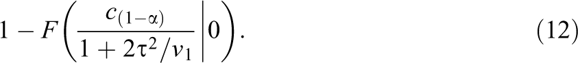
Consider designing Study 2 (the replicate) to ensure a sufficiently powered test. As in the studies-fixed case, suppose that we observe Study 1, which has true effect size $θ_{1} > 0$ and estimation error variance v₁. Because v₁ is fixed, it is clear that the maximum power of the test is bounded below one for a given (finite) τ². Letting v₂ tend to zero so that Study 2 has an indefinitely large sample size, we see that the maximum power would be

1 - F (\frac{c_{(1 - α)}}{1 + 2 τ^{2} / v_{1}} | 0) .

The power in Equation 12 is an increasing function of τ². This means the highest power this test could have depends on the maximum value of τ² (call this $τ_{N}^{2}$ ) that could be considered negligible. We would argue that $τ_{N}^{2}$ is the value of τ² that makes large differences between $θ_{1}$ and θ₂ unlikely. Let δ² = (θ₁ − θ₂)² be the squared difference between effect parameters, $δ_{0}^{2}$ be the largest value of δ² considered negligible, and 1 − γ be the probability that $δ^{2} < δ_{0}^{2}$ . Then, we can formalize this idea in terms of the following inequality:

P {{(θ_{1} - θ_{2})}^{2} < δ_{0}^{2}} < 1 - γ.

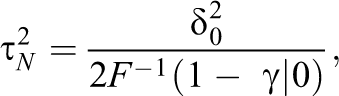
Assume that $θ \sim N (μ, τ^{2})$ , the usual assumption in the random effects model, then the corresponding value of $τ_{N}^{2}$ that satisfies Equation 13 is given by

τ_{N}^{2} = \frac{δ_{0}^{2}}{2 F^{- 1} (1 - γ| 0)},

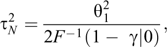
where F(x | 0) is the χ² distribution function as in Equation 2. Note that $τ_{N}^{2}$ is an increasing function of $δ_{0}^{2}$ , and so we may write it as $τ_{N}^{2} (δ_{0}^{2})$ . As argued in the previous sections, we would consider $δ_{0}^{2} < θ_{1}^{2}$ , which corresponds with qualitative agreement between θ₁ and θ₂, to be an upper bound for a negligible difference between effect parameters. This would imply that

τ_{N}^{2} = \frac{θ_{1}^{2}}{2 F^{- 1} (1 - γ| 0)},

is the largest value of τ² we could consider negligible. Substituting this into Equation 12, we see that the most sensitive design would give a maximum power of

1 - F (\frac{F^{- 1} (1 - γ | 0) c_{(1 - α)}}{F^{- 1} (1 - γ | 0) + θ_{1}^{2} / v_{1}} | 0) .

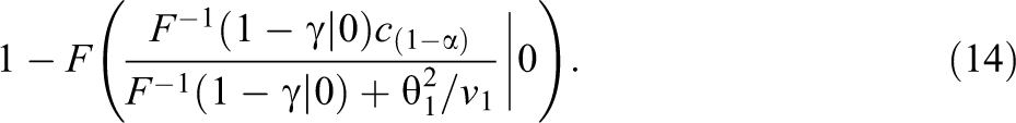
Note that Equation 14 increases with the power of Study 1 to detect a nonnull effect (i.e., $θ_{1}^{2} / v_{1}$ ). It also decreases with the proportion of studies required to be qualitatively consistent with θ₁ (i.e., 1 − γ), since if we require a smaller proportion of replications to be consistent with θ₁, then we would consider larger values of $τ^{2}$ to be negligible.

What is a reasonable proportion γ? Choosing γ = 24%, so that more than 75% of the θ values are consistent with $θ_{1}$ , yields $τ_{N}^{2} = θ_{1}^{2} / 2.76$ . Given that value of γ, the maximum power of the test for replication (i.e., when v₂ = 0) depends on the power of Study 1 to find a nonnull effect (via $θ_{1}^{2} / v_{1}$ ). If Study 1 has 80% power to detect a nonnull effect (so $θ_{1}^{2} / v_{1} = 7.85$ ), the random effects test for exact replication will have power less than 45% (assuming v₂ = 0). If $θ_{1}^{2} / v_{1} = 7.85$ and Study 2 has a finite sample size such that v₂ = v₁ or v₂ = v₁/2, then the power of the test would be 31% and 37%, respectively. One could choose different values of γ, but no plausible values imply that the test for replication has higher power than the original study.

It is worth noting that as with the fixed effects tests, random effects tests that need to adjust for publication selection will be less powerful than tests that do not need to make such adjustments. This is because the power of the random-studies tests depends entirely on and is an increasing function of τ²/(v₁ + v₂). However, if publication bias corrections are required, then rather than using v₁, the test now involves the corrected estimation error variance $v_{1}^{*}$ . Recall that $v_{1} < v_{1}^{*}$ , which means that $τ^{2} / (v_{1} + v_{2}) > τ^{2} / (v_{1}^{*} + v_{2})$ . Therefore, if the test must account for publication bias, it will be even less powerful than the one that does not.

Random Effects Test for Approximate Replication

The studies-random test for approximate replication requires the specification of the largest negligible heterogeneity in terms of the between-studies variance of effect parameters. Call this variance $τ_{0}^{2}$ . Thus, the null hypothesis of approximate replication is not $τ_{0}^{2} = 0$ (as in exact replication) but

H_{0} : τ^{2} \leq τ_{0}^{2} .

To test this hypothesis at significance level α using the Q-statistic, the reference distribution is that of Q when $τ^{2} = τ_{0}^{2}$ , so that the test rejects the null hypothesis of approximate replication when Q exceeds the 100(1 − α) percentile of the distribution of Q when $τ^{2} = τ_{0}^{2}$ . Call this critical value $c_{(1 - α)} {(τ}_{0}^{2})$ to emphasize its dependence on $τ_{0}^{2}$ . Using Equation 7, the value of $c_{(1 - α)} {(τ}_{0}^{2})$ can be obtained from $c_{(1 - α)}$ as

c_{(1 - α)} (τ_{0}^{2}) = (1 + \frac{2 τ_{0}^{2}}{v_{1} + v_{2}}) c_{(1 - α)},

which is larger than $c_{(1 - α)}$ . Thus, the power of the level α test for approximate replication under the studies-random model is

1 - F (\frac{c_{(1 - α)} (τ_{0}^{2})}{1 + 2 τ^{2} / (v_{1} + v_{2})} | 0),

where F(x | 0) is the cumulative distribution function of the (central) χ² distribution with one degree of freedom. The only difference between the expression for statistical power of the test for approximate replication Equation 16 and that of the test of exact replication Equation 12 is the critical value each uses. As with the fixed-studies model, tests for approximate replication will be less powerful than those of exact replication, and they will be even less powerful if they must correct for publication bias. Therefore, if tests for exact replication based on a single study are insufficiently powerful, so are tests for approximate replication.

Random Effects Tests for Nonreplication

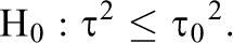
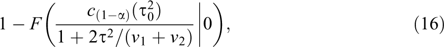
The random effects test for nonreplication involves a null hypothesis that the studies failed to replicate. Operationalizing this requires some idea about the smallest value of $τ_{0}^{2}$ that could be considered nonnegligible. The null hypothesis is given by $H_{0} : τ^{2} \geq τ_{0}^{2} .$

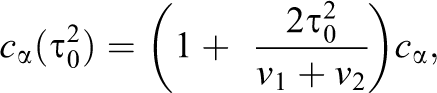
To test H₀, compute Q as in Equation 1 and compare it to $c_{α} {(τ}_{0}^{2})$ , the 100α percent point of the random-studies distribution of Q when $τ^{2} = τ_{0}^{2}$ :

c_{α} (τ_{0}^{2}) = (1 + \frac{2 τ_{0}^{2}}{v_{1} + v_{2}}) c_{α},

where c_α is the 100α percentile of the central χ² distribution with one degree of freedom. We reject H₀ and conclude that the studies replicate if Q is less than $c_{α} (τ_{0}^{2})$ .

For $τ^{2} < τ_{0}^{2}$ , the power of this test is given by

F (\frac{c_{α} (τ_{0}^{2})}{1 + 2 τ^{2} / (v_{1} + v_{2})} | 0),

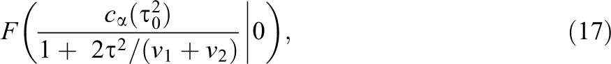
where F(x | 0) is the (central) χ² distribution function with one degree of freedom. Note that the power increases as τ² decreases, and attains a maximum at τ² = 0. Likewise, the power also increases as $τ_{0}^{2} / (v_{1} + v_{2})$ increases, and attains a maximum when v₂ tends to be zero (i.e., if Study 2 has an infinite sample size). Thus, the maximum power of this test is given by

F [(1 + 2 \frac{τ_{0}^{2}}{v_{1}}) c_{α} | 0] .

An upper bound of $τ_{0}^{2}$ worth testing can be obtained using a similar approach to the previous section, where we choose a value of $τ_{0}^{2}$ that corresponds with a given percentage (denoted 1 − γ) of replications being consistent with θ₁. Using Equation 13, we would argue an upper bound of the power of this test would be

F [(1 + \frac{θ_{1}^{2}}{v_{1}} \frac{1}{F (1 - γ | 0)}) c_{α} | 0] = F [(1 + \frac{λ_{1}}{F (1 - γ | 0)}) c_{α} | 0] .

The maximum power in Equation 19 increases with the power of Study 1 (via $θ_{1}^{2} / v_{1}$ ) and decreases with the proportion of studies required to be consistent (1 − γ). If Study 1 has 80% power, then setting γ = 25% in Equation 13 would mean that a quarter of potential replications would be inconsistent with θ₁ and would give a test for nonreplication with power less than 13%. Note that even if Study 1 has 90% power, the power for the test of nonreplication would be less than 15% for γ = 25%. Alternatively, if we use γ = 50%, so that half of the potential replications would be inconsistent with θ₁, the maximum power would be below 21% (assuming Study 1 had 80% power). Indeed, to even approach a maximum power greater than 50% would require γ = 80%, so that 80% of replications would be inconsistent with θ₁; however, this would seem to be too lax a definition of nonreplication to be practical.

If the analysis must correct T₁ for publication bias, then the test uses $v_{1}^{*}$ the variance of the corrected estimate instead of v₁. Note that the power of the test for nonreplication given in Equation 17 increases as τ²/(v₁ + v₂) decreases and that $τ^{2} / (v_{1} + v_{2}) > τ^{2} / (v_{1}^{*} + v_{2}) > 0$ . However, the maximum possible power in Equation 19 sets τ²/(v₁ + v₂) = 0 and thus serves as an upper bound even in the face of publication bias corrections.

Estimation of Heterogeneity Parameters

An alternative way to assess heterogeneity is to estimate a parameter that characterizes the difference among the $θ_{i}$ . When studies are considered fixed, the only $θ_{i}$ relevant to evaluating replication are $θ_{1}$ and $θ_{2}$ , the effect size parameters in the observed studies. In this case, an appropriate parameter characterizing difference among the $θ_{i}$ is some function of $θ_{1} - θ_{2}$ . Recall that the noncentrality parameter that determines the distribution of Q is

λ = {(θ_{1} - θ_{2})}^{2} / (v_{1} + v_{2}) = {(θ_{1} - θ_{2})}^{2} / 2 \bar{v},

where $\bar{v} = (v_{1} + v_{2}) / 2$ is the average variance. Thus, λ has merit as a scale-free parameter characterizing heterogeneity. Because Q has the noncentral χ² distribution with one degree of freedom and noncentrality parameter λ when $θ_{1} \neq θ_{2}$ , and the expected value of Q is 1 + λ, it follows that

\hat{λ} = Q - 1,

is an unbiased estimator of λ, with SE

S E {\hat{λ}} = \sqrt{2 (1 + 2 λ)} .

Note that the SE is always larger than 1.41 (which occurs when λ = 0) and it is an increasing function of λ (e.g., it is 2.45 when λ = 1). For the conventions of negligible heterogeneity, the SE of this estimate is 1.73 (when λ = 1/4), 1.83 (when λ = 1/3), and 2.16 (when λ = 2/3). In other words, the SE of the estimator afforded by the design involving a single replication study is several times larger than the true values that are likely to be of interest.

This remains true if the estimate adjusts for publication bias in Study 1. In that case, the estimator in Equation 20 uses the values of the corrected estimate $T_{1}^{*}$ and its variance $v_{1}^{*}$ rather than T₁ and v₁. Since $v_{1} < v_{1}^{*}$ , it follows that $λ^{*} = {(θ_{1} - θ_{2})}^{2} / (v_{1}^{*} + v_{2})$ is smaller than $λ = {(θ_{1} - θ_{2})}^{2} / (v_{1} + v_{2})$ . This means that if Study 1 is subject to publication selection, both the quantity being estimated λ* and its SE will be smaller than if there was no publication selection. However, the SE will still be very large relative to meaningful values of λ* we would want to estimate precisely. As we saw above, we may want our analysis to be sensitive to values of λ (and hence λ*) that are less than one. Standard errors of estimates of λ* in that range are no smaller than 1.41 (which occurs if λ* = 0). Thus, we will be unable to obtain precise estimates of meaningful values of λ or λ* with only two studies.

When studies are considered random, the entire distribution of $θ_{i}$ in the universe from which the observed studies are sampled is relevant to evaluating replication. In this case, an appropriate parameter to characterize differences among the $θ_{i}$ is τ², technically the variance of the effect size parameters in the population from which the studies are a sample. There are several ways to estimate τ², but the method most often used in meta-analysis (the DerSimonian and Laird method) is based on the Q-statistic. When k = 2, that estimate of τ² is

{\hat{τ}}^{2} = (Q - 1) (v_{1} + v_{2}) / 2,

which is an unbiased estimate of τ² under the model (see, e.g., Hedges & Pigott, 2001). (The estimate can be negative and when this is so, the estimate is usually truncated to zero.) The variance of the estimate of τ² given in Equation 22 is

S E {{\hat{τ}}^{2}} = \sqrt{2} [(v_{1} + v_{2}) / 2 + τ^{2}] = \sqrt{2} [\bar{v} + τ^{2}] > τ^{2},

where $\bar{v} = (v_{1} + v_{2}) / 2$ . If Study 1 is adjusted for publication bias, we can rewrite Equation 23 using $\bar{v} \equiv {\bar{v}}^{*} = (v_{1}^{*} + v_{2}) / 2$ , and it remains true that the SE of the estimate of τ² is greater than τ² itself.

Note however that τ² is not necessarily scale-free. It is in the same units as the effect size θ, and when θ is not scale-free (e.g., if it is an unstandardized mean difference), τ² will not be scale-free. Dividing τ² by $\bar{v} = (v_{1} + v_{2}) / 2$ results in a scale-free parameter characterizing heterogeneity similar to λ with SE given by

S E {{\hat{τ}}^{2} / \bar{v}} = \sqrt{2} [1 + τ^{2} / \bar{v}] > τ^{2} / \bar{v} .

If the effect size in Study 1 must be corrected for publication bias, Equation 24 can be rewritten by substituting ${\bar{v}}^{*}$ for $\bar{v}$ .

Both Equations 23 and 24 show that whether we are interested in estimating τ² or $τ^{2} / \bar{v}$ , the SE afforded by the design of two studies (regardless of whether the estimate in one of the studies must correct for publication bias) will necessarily always be greater than the magnitudes that are of interest. Recall that the conventional definitions of negligible heterogeneity that we cited from physics, personnel psychology, and medicine were fractions $τ^{2} / v$ and the largest fraction was 2/3. The SE of $\hat{λ}$ or ${\hat{τ}}^{2} / \bar{v}$ estimated from two studies is therefore more than twice as large as the largest of these conventions.

Regardless of whether studies are considered fixed or considered random, the uncertainty of the heterogeneity parameter being estimated is very large in comparison to important values of the parameter itself. Thus, evaluation of replication via estimation is not sufficiently sensitive to obtain unambiguous conclusions when there is only a single replication study.

Comparing an Original Study to the Mean of Several Others Does Not Resolve the Sensitivity Problem

It might seem that, if one replication study is inadequate to yield a statistical analysis with adequate sensitivity, the obvious solution is to carry out more replication studies and compare the replication studies to the original study. Such analyses (often called subgroup analyses or fitting categorical models to effect sizes) are standard part of meta-analysis (see chapter 7 of Hedges & Olkin, 1985). However, such a strategy is mathematically equivalent to combining the estimates from all of the replication studies into one “synthetic study” and computing an effect size estimate (and its variance) from that synthetic replication study. The analysis of the difference between the original study and the synthetic replication study is subject to exactly the same limitations of analyses comparing two studies that are described in this article.

Greater sensitivity (higher power or greater precision in heterogeneity parameter estimates) can be achieved with additional studies, but only by redefining the focus of the analysis to be on the heterogeneity of all studies (see Hedges & Schauer, 2018). This means that the original study is not privileged in the interpretation and that differences among the effects of all the studies (original and replication studies) are treated as equally relevant in evaluating replication.

Such analyses can be carried out using the Q-statistic, and experience with such analyses is the source of the conventions mentioned previously that emerged in physics, personnel psychology, and medicine. Methods for carrying out relevant power analyses described here were given by Hedges and Pigott (2001). Power analysis can be an important tool for use in the design of ensembles of studies to carry out empirical evaluations of replication. Although the details are slightly different, the power of either fixed or random effects tests based on the Q-statistic depends on the amount of heterogeneity among parameters (e.g., τ²), the number of studies (k), and the estimation error variance of the effects (v, which will typically depend on sample size n, in each study). Given a fixed amount of heterogeneity (e.g., fixed τ²), power can be increased by increasing k or increasing n (which decreases v). One design problem is how to choose n and k to produce a design that will be both feasible and sensitive enough to yield unambiguous conclusions. One might even want to posit a cost function and attempt to find optimal designs (e.g., designs that obtain a given power or precision of estimates for the smallest cost).

Alternative Perspectives on Replication

We have argued that the definition of replication ought to focus on the similarity between effect parameters θ₁ and θ₂ and that replications should be designed to support unambiguous conclusions about that definition. However, this article has shown that it is unlikely that analyses of replication based on only two studies will be adequately sensitive to differences between θ₁ and θ₂. This is not necessarily a limitation of the methods. The Q-test is the likelihood ratio test under the model and is thus the uniformly most powerful unbiased test, meaning that no other test of the similarity of θ₁ and θ₂ will be more powerful.

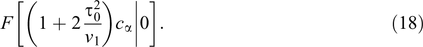
It would be tempting to view this merely as a limitation of frequentist analysis methods. While we agree that the Bayesian approach has certain interpretational advantages (e.g., it can characterize the probability distribution of $θ_{1} - θ_{2}$ ), it does not obviate the essential problem that two studies, even if conventionally well powered, do not provide enough information to allow a sensitive analysis of replication. Bayesian approaches that assess the same operational definition of replication as the frequentist methods in this article might focus on estimating the difference between θ₁ and θ₂. One way to conceive of sensitivity of such analyses is via the width of the 95% posterior credible intervals.

For example, suppose that we assume that $θ_{1} - θ_{2}$ has a normal prior distribution with variance v_P. Then, the posterior distribution of $θ_{1} - θ_{2}$ given T₁ − T₂ is normal with variance v_P(v₁ + v₂)/(v_P + v₁ + v₂). If we write v_P = (v₁ + v₂)/α, then α can be interpreted as the strength of prior information in units of the pair of studies that provide data. Thus, if the prior information is equivalent to the observed pair studies, α = 1, if the prior provides less information than the observed studies, α < 1. The posterior variance σ² reduces to

σ^{2} = \frac{v_{1} + v_{2}}{α + 1} .

To say that the prior is relatively uninformative is to say that v_P > v or that α is considerably less than one. If the prior had one fifth of the information in the two studies (α = 1/5), the posterior standard deviation would be 91% as large as the frequentist variance of T₁ − T₂; if the prior had one tenth as much information as the two studies, the posterior standard deviation would be 95% as large as the frequentist variance of T₁ − T₂. In other words, if the prior is relatively uninformative, the length of the corresponding posterior intervals and confidence intervals would be very similar.

This has important implications for the frequentist performance of the posterior interval. The 95% posterior credible interval is

T_{1} - T_{2} \pm 1.96 \sqrt{\frac{v_{1} + v_{2}}{α + 1}} .

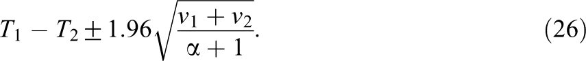
Because T₁ − T₂ is normally distributed with variance v₁ + v₂, if the mean of T₁ − T₂ were actually zero, the probability that the upper credible value U exceeds any point c would be

P {U > c} = 1 - Φ (\frac{c}{\sqrt{v_{1} + v_{2}}} - \frac{1.96}{\sqrt{α + 1}}) .

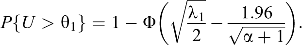
One way to evaluate this posterior credible interval is ask how often the upper credible value U exceeds a nonnegligible value of $θ_{1} - θ_{2}$ . We argued before that consistency of sign $(0 < θ_{2} < θ_{1})$ was one sensible definition of the largest negligible difference. If $θ_{1} = 0.5$ , a posterior value of $θ_{1} - θ_{2} \geq 0.5$ would correspond to a nonnegligible difference, and hence, it would be of interest how probable U was to exceed 0.5. Suppose that Study 1 has a preset level of statistical power, which defines a value of $λ_{1} = θ_{1}^{2} / v_{1}$ . Setting $c = θ_{1} = \sqrt{λ_{1} v_{1}}$ and assuming v₁ = v₂, so that the original and replication study have equal precision (27) implies that

P {U > θ_{1}} = 1 - Φ (\sqrt{\frac{λ_{1}}{2}} - \frac{1.96}{\sqrt{α + 1}}) .

If the prior is even remotely uninformative, it turns out that U will often exceed θ₁. For instance, let α ≤ 0.1 with θ₁ = θ₂ and v₁ = v₂, so that both studies are reasonably well powered and the prior contains about one tenth of the information of both studies, then $P {U > θ_{1}} > 45 %$ . Even if v₂ = v₁/10, so that Study 2 is 10 times the size as Study 1, $P {U > θ_{1}} > 21 %$ for α ≤ 0.1. Greater precision can be introduced with a more informative prior. But when v₁ = v₂, so that both studies have 80% power, even when α = 1, so that the prior contains as much information as both studies, $P {U > θ_{1}} > 27 %$ . This suggests that the posterior credible interval would be unlikely to provide an unambiguous means of evaluating replication when there are two studies. Like the frequentist methods, performance would be better if there were more studies or if both individual studies provided more information (e.g., had larger sample sizes).

Other forms of argumentation have been offered to do analyses about replication. For example, Hartgerink, Wicherts, and van Assen (2017) formalize how Fisher’s method can be used to examine potential errors in frequentist determinations about replication, and Simonsohn (2015) proposes assessing the relative sensitivity of each study. Etz and Vandekerckhove (2016) evaluate the strength of evidence regarding whether effects are nonzero in the original and replication studies using Bayes factors. van Aert and van Assen (2017) assume that the studies replicate exactly and pool information across original and replication studies.

Each of the methods discussed in the previous paragraph assesses replication using a fundamentally different operational definition. For instance, seemingly successful replications in Etz and Vandekerckhove’s analysis involve both the original and replication studies showing “strong evidence of an effect.” This would mean that there is convincing evidence that both θ₁ ≠ 0 and θ₂ ≠ 0, but this definition of replication puts no restriction on how different θ₁ and θ₂ can be. Conversely, van Aert and van Assen’s analyses assume that the studies replicated exactly, so that θ₁ = θ₂. In either case, any gains in information come at the cost of much looser definitions of replication or in much stronger assumptions. Moreover, precisely what is gained in terms of information (and what is lost in interpretability) for these Bayesian methods does not appear to have been studied, particularly in relation to design.

Conclusions

It might seem that there is nothing special about the design of a replication study. If there is an existing study, simply plan one more study so that it will provide the required sensitivity in the analysis of replication. We have shown that an ensemble of two studies (the original and one replicate) typically cannot provide a test for replication that has high power or an estimate of heterogeneity parameters with high precision (small SE). This finding is consistent with the conclusion of Maxwell, Lau, and Howard (2015) that high power tests of replication are difficult to obtain, but even stronger. A single replication study usually cannot provide adequate sensitivity to evaluate replication without ambiguity.

The exceptions to this argument would be cases in which the original study had very high statistical power and was not subject to publication bias. Surveys of statistical power suggest that very high statistical power is unlikely in most psychological research (see, e.g., Dumas-Mallet et al., 2017; Vankov et al., 2014). While the degree of publication bias is difficult to confirm, prospective studies suggest the widespread existence of publication bias (see, e.g., Dickersin, 2005). The ubiquity of statistically significant results coupled with the low estimated power of studies in the literature also supports the existence of publication bias.

The results of this article suggest that the statistical aspects of the design of (ensembles of) replication studies deserve greater attention than it has received. In most situations, single replication studies are inadequate to yield sufficiently sensitive analyses (and therefore unambiguous findings), so designs with more than one replication study are needed. Methods for testing replication in such designs and for assessing their sensitivity are available (see Hedges & Schauer, 2018). Although it appears that adequate sensitivity can usually be achieved with enough replication studies, this statement is not a detailed solution to the design problem, any more than saying a large enough sample size can usually yield adequate power is a solution to the problem of design of single experiments.

Finally, while the findings of this article suggest that conducting only a single replication study is not a sensitive research design that does not mean that a replication study lacks value. A single replication adds to the total information there is about an effect and the average of the two effects effect is likely to have more information (smaller SE) than the estimate from the initial study. It can also give useful insight into protocol standardization, suggest avenues of future innovation, and provide additional insight for making evidence-based policy. Moreover, a single initial replication may be one effort in a sequence of replications, and as researchers conduct additional subsequent replications, eventually a preponderance of evidence will support more sensitive analyses. Finally, the role of conducting a replication, particularly a conceptual replication, may not even be to get the same result as an original study, but instead to investigate the how a finding changes in new settings or under different conditions.

Footnotes

Declaration of Conflicting Interests

The author(s) declared no potential conflicts of interest with respect to the research, authorship, and/or publication of this article.

Funding

The author(s) disclosed receipt of the following financial support for the research, authorship, and/or publication of this article: Institute of Education Sciences (R305B140042), Institute of Education Sciences (R305D140045), and National Science Foundation (1841075).

ORCID iD

Jacob M. Schauer

References

Baker

. (2016). 1,500 scientists lift the lid on reproducibility. Nature, 533, 452–454.

Camerer

C. F.

Dreber

Forsell

T. H.

Huber

Johannesson

… Wu

(2016). Evaluating the reproducibility of laboratory experiments in economics. Science, 351, 1433–1436.

Cohen

(1977). Statistical power analysis for the behavioral sciences (2nd ed.). New York, NY: Academic Press.

Collins

F. S.

Tabak

L. A.

(2014). NIH plans to enhance reproducibility. Nature, 505, 612–613.

Collins

H. M.

(1992). Changing order: Replication and induction in scientific practice. Chicago, IL: University of Chicago Press.

Cooper

H. M.

Hedges

L. V.

Valentine

(2009). The handbook of research synthesis and meta-analysis (2nd ed.). New York, NY: The Russell Sage Foundation.

Dickersin

(2005). Publication bias: Recognizing the problem, understanding its origins and scope, and preventing harm. In Rothstein

H. R.

Sutton

A. J.

Borenstein

(Eds.), Publication bias in meta-analysis: Prevention, assessment, and adjustments (pp. 11–33). Chichester, England: Wiley.

Dumas-Mallet

Button

K. S.

Boraud

Gonon

Munafò

M. R.

(2017). Low statistical power in biomedical science: A review of three human research domains. Open Science, 4, 160254.

Etz

Vandekerckhove

(2016). A Bayesian perspective on the reproducibility project: Psychology. PLOS One, 11, e0149794. doi:10.1371/journal.pone.0149794

10.

Gelman

Stern

(2006). The difference between “significant” and “not significant” is not itself statistically significant. American Statistician, 60, 328–331.

11.

Gilbert

D. T.

King

S. G.

Pettigrew

Wilson

T. D.

(2016). Comment on “Estimating the reproducibility of psychological science.” Science, 351, 1037–1038.

12.

Gomez

O. S.

Juristo

Vargas

(2010). Replications types in experimental disciplines. ESEM, 10.

13.

Hartgerink

C. H. J.

Wicherts

J. M.

van Assen

M. A. L. M

. (2017). Too good to be false: Nonsignificant results revisited. Collabra: Psychology, 3, 9. doi:10.1525/collabra.71

14.

Hedges

L. V.

(1984). Estimation of effect size under nonrandom sampling: The effects of censoring studies yielding statistically insignificant mean differences. Journal of Educational Statistics, 9, 61–85.

15.

Hedges

L. V.

(1987). How hard is hard science, how soft is soft science? The empirical cumulativeness of research. American Psychologist, 42, 443–455.

16.

Hedges

L. V.

Olkin

(1980). Vote-counting methods in research synthesis. Psychological Bulletin, 88, 359–369.

17.

Hedges

L. V.

Olkin

(1985). Statistical methods for meta-analysis. New York, NY: Academic Press.

18.

Hedges

L. V.

Pigott

T. D.

(2001). The power of statistical tests in meta-analysis. Psychological Methods, 6, 203–217.

19.

Hedges

L. V.

Schauer

. (2018). Statistical analyses for studying replication: Meta-analytic perspectives. Psychological Methods. Advance online publication. Retrieved from https://dx-doi-org.web.bisu.edu.cn/10.1037/met0000189

20.

Hedges

L. V.

Vevea

J. L.

(1998). Fixed and random effects models in meta-analysis. Psychological Methods, 3, 486–504.

21.

Higgins

J. P. T.

Green

(2008). The Cochrane handbook for systematic reviews of interventions. Chichester, England: John Wiley.

22.

Humphreys

L. G.

(1980). The statistics of failure to replicate: A comment on Buriels (1978) conclusions. Journal of Educational Psychology, 72, 71–75.

23.

Hunter

J. E.

Schmidt

F. L.

(1990). Methods of meta-analysis: Correcting error and bias in research findings. Newbury Park, CA: Sage.

24.

Ioannidis

J. P. A.

(2005). Contradicted and initially stronger effects in highly cited clinical research. Journal of the American Medical Association, 294, 218–228.

25.

Lykken

D. T.

(1968). Statistical significance in psychological research. Psychological Bulletin, 70, 151–159.

26.

Maxwell

S. E.

Lau

M. Y.

Howard

G. S.

(2015). Is psychology really suffering from a replication crisis? American Psychologist, 70, 487–498.

27.

McNutt

(2014). Reproducibility. Science, 343, 229.

28.

McShane

B. B.

Böckenholt

Hansen

K. T.

(2016). Adjusting for publication bias in meta-analysis: An evaluation of selection methods and some cautionary notes. Perspectives on Psychological Science, 11, 730–749. doi:10.1177/1745691616662243

29.

Olive

K. A.

Particle Data Group . (2014). Review of particle properties. Chinese Physics Journal C, 38, 090001. Retrieved from http://iopscience.iop.org/issue/1674-1137/38/9

30.

Open Science Collaborative. (2015). Estimating the reproducibility of psychological science. Science, 349, 943–951.

31.

Pashler

Harris

C. R.

(2012). Is the replicability crisis overblown? Three arguments examined. Psychological Science, 7, 531–536.

32.

Perrin

(2014). Make mouse studies work. Nature, 507, 423–425.

33.

Rosenfeld

(1975). The particle data group: Growth and operations. Annual Review of Nuclear Science, 555–559.

34.

Rothstein

Sutton

A. J.

Borenstein

(2005). Publication bias in meta-analysis: Prevention, assessment and adjustments. Hoboken, NJ: Wiley.

35.

Schmidt

(2009). Shall we really do it again? The powerful concept of replication is neglected in the social sciences. Review of General Psychology, 13, 90–100.

36.

Sidman

(1960). Tactics of scientific research. Oxford, England: Basic Books.

37.

Simonsohn

(2015). Small telescopes: Detectability and the evaluation of replication results. Psychological Science, 26, 559–569.

38.

Steiner

P. M.

Wong

V. C.

(2018). Replication designs for causal inference (Working Paper No. 62). Retrieved from https://curry.virginia.edu/sites/default/files/uploads/epw/62_Replication_Designs.pdf

39.

van Aert

R. C. M.

van Assen

M. A. L. M.

(2017). Bayesian evaluation of effect size after replicating an original study. PLOS One, 12, e0175302. Retrieved from https://doi.org/10.1371/journal.pone.0175302

40.

Vankov

Bowers

Munafò

M. R.

(2014). On the persistence of low power in psychological science. The Quarterly Journal of Experimental Psychology, 67, 1037–1040.