
Abstract
Causal effects are commonly defined as comparisons of the potential outcomes under treatment and control, but this definition is threatened by the possibility that either the treatment or the control condition is not well defined, existing instead in more than one version. This is often a real possibility in nonexperimental or observational studies of treatments because these treatments occur in the natural or social world without the laboratory control needed to ensure identically the same treatment or control condition occurs in every instance. We consider the simplest case: Either the treatment condition or the control condition exists in two versions that are easily recognized in the data but are of uncertain, perhaps doubtful, relevance, for example, branded Advil versus generic ibuprofen. Common practice does not address versions of treatment: Typically, the issue is either ignored or explicitly stated but assumed to be absent. Common practice is reluctant to address two versions of treatment because the obvious solution entails dividing the data into two parts with two analyses, thereby (a) reducing power to detect versions of treatment in each part, (b) creating problems of multiple inference in coordinating the two analyses, and (c) failing to report a single primary analysis that uses everyone. We propose and illustrate a new method of analysis that begins with a single primary analysis of everyone that would be correct if the two versions do not differ, adds a second analysis that would be correct were there two different effects for the two versions, controls the family-wise error rate in all assertions made by the several analyses, and yet pays no price in power to detect a constant treatment effect in the primary analysis of everyone. Our method can be applied to analyses of constant additive treatment effects on continuous outcomes. Unlike conventional simultaneous inferences, the new method is coordinating several analyses that are valid under different assumptions, so that one analysis would never be performed if one knew for certain that the assumptions of the other analysis are true. It is a multiple assumptions problem rather than a multiple hypotheses problem. We discuss the relative merits of the method with respect to more conventional approaches to analyzing multiple comparisons. The method is motivated and illustrated using a study of the possibility that repeated head trauma in high school football causes an increase in risk of early onset cognitive decline.
Keywords
1. What Are Versions of Treatment?
Commonly, the effect on an individual caused by a treatment is defined as a comparison of the two potential outcomes that this individual would exhibit under treatment and under control (see Neyman, 1923/1990; Rubin, 1974; Welch, 1937). Implicit in this definition is the notion that the treatment and control conditions are each well defined. In particular, it is common to assume that there are “no versions of treatment or control” (see Rubin, 1986).
By definition, versions of treatment are not intended additions to a study design, but rather potential flaws in the study design. Versions of treatment or control are often associated with finding treatments that occur naturally, rather than experimentally manipulating a tightly controlled, uniform treatment. Versions of one treatment should be distinguished from the intentional study of distinct, competing treatments. When an investigator discusses versions of one treatment, she is expressing a preference for the conception that there is a single treatment but is acknowledging the possibility that her preferred conception is mistaken. Branded Advil and generic ibuprofen are versions of one treatment—possibly different, but very plausibly expected to be the same—whereas ibuprofen and aspirin are different competing treatments. The investigator and her audience prefer a primary analysis that does not distinguish versions of treatment, but both would be reassured by evidence that showed their preferred analysis does not embody a consequential error. Versions of control groups should also be distinguished from the deliberate use of two carefully selected control groups intended to reveal unmeasured biases if present (see, for instance, Rosenbaum, 1987). In particular, Campbell (1969) suggested that two control groups should be deliberately selected to systematically vary a specific unmeasured covariate in an effort to demonstrate its irrelevance; however, versions of control are unintended flaws in study design, not purposeful quasi-experimental devices.
There are two versions of either the treatment condition or the control condition if we recognize in available data either two types of treated subjects or two types of controls, but we are uncertain about, or perhaps explicitly doubt, the relevance of this visible distinction. Versions refer to a visible but perhaps unimportant distinction, not to a distinction that is hidden or latent. There are important methodological issues in recognizing treatments that inexplicably affect some people but not others; however, this is practically and mathematically a different problem (Conover & Salsberg, 1988; Rosenbaum, 2007a).
In discussing randomized clinical trials, Peto et al. (1976, pp. 590–591) wrote,
A positive result is more likely, and a null result is more informative, if the main comparison is of only 2 treatments, these being as different as possible.…[I]t is a mark of good trial design that a null result, if it occurs, will be of interest.
This advice is equally relevant for observational studies, and it is part of the reason that we prefer a conception in which there is a single treated condition and a single control condition. Despite this, an investigator may seek some reassurance that the study’s conclusions cannot be undermined by the possibility of two versions of treatment.
In that spirit, our analysis focuses on the main treatment–control comparison and subordinates the study of versions of treatment or versions of control. In particular, the main treatment–control comparison is unaffected by the exploration of versions of treatment—the usual confidence interval for a constant effect is reported—despite controlling the family-wise error rate in multiple comparisons that explore the possibility of versions of treatment with different effects. Two confidence intervals are reported, the usual interval for a constant effect and an interval designed to contain both effects if the two versions differ. If the effect is constant, then both intervals simultaneously cover that one effect with probability
2. Possible Versions of Control in a Study of Football and Dementia
There is evidence that severe repeated head trauma accelerates the onset of cognitive decline or dementia (Graves et al., 1990; Mortimer et al., 1991), with specific concern about the risks faced by professional football players and boxers (Lehman et al., 2012; McKee et al., 2009). It is unclear whether there is also increased risk from playing football on a team in high school, but there have been several recommendations against tackle football in high school (Bachynski, 2016; Miles & Prasad, 2016). Does high school football accelerate the onset of cognitive decline?
A recent investigation used data from the Wisconsin Longitudinal Study, comparing cognition and mental health measured at ages 65 and 72, recorded in 2005 and 2011, of men who played football on a high school team in the mid-1950s to male controls of similar age who did not play football (Deshpande et al., 2017). Following the practice in clinical trials, and as is recommended for observational studies by Rubin (2007), the design and protocol for this study were published online after matching was completed but before outcomes were examined (Deshpande et al., 2016). The small number of people who engaged in sports other than football with high incidences of head trauma such as soccer, hockey, and wrestling were excluded from both the football and control groups. One outcome was the 0 to 10 score on a 10-item delayed word recall (DWR) test at ages 65 and 72. The DWR test was designed as an inexpensive measure of memory loss associated with dementia (see Knopman & Ryberg, 1989). In this test, a person is asked to remember a list of words that is then read to the person. Attention then shifts to another activity, and after a delay, the person is asked to recall as many words from the list as possible. The DWR score is the number of words remembered. On average, in the Wisconsin Longitudinal Study, performance on the DWR test declined by half a word from age 65 to 72. It is useful to keep that half-word, 7-year decline in mind when thinking about the magnitude of the effect of playing football.
A comparison of football players to all controls is natural and might be conducted without second thought. Among the controls, however, some played a noncollision sport-like baseball or track, while others played no sports at all. An investigator might reasonably seek reassurance that this natural comparison has not oversimplified these two version of “not playing football.” At the same time, the investigator does not want to sacrifice power to detect a constant treatment effect in the main comparison en route to obtaining this reassurance by subdividing the data into many slivers of reduced sample size and correcting for multiple comparisons. The method we propose achieves both of these objectives.
Our question concerns the effects of high school football. It is important to distinguish this question from questions about the effects of severe head trauma in general. It is at least conceivable that high school football is comparatively harmless, while severe head trauma is not, simply because severe head trauma is not common in high school football, and the benefits of exercise for all football players offset the harm of severe but rare trauma. Conversely, severe head trauma from automotive or other accidents may be difficult to prevent, but if high school football had grave consequences, then it could simply be banned, in the same way that most high schools do not have boxing teams. We ask about the effects of playing football in high school on subsequent cognitive function.
The Wisconsin Longitudinal Study describes a specific piece of the United States over a specific period of time, and caution is advised about extrapolating its conclusions to other times and places. High School football may have changed since the 1950s, and the demographic composition of Wisconsin in the 1950s is not the demographic composition of the United States. The Wisconsin Longitudinal Study is primarily a sequence of surveys, and it is impossible to use it to investigate questions not asked in those surveys. For instance, we cannot identify high school students who went on to play professional football, but we suspect they were few in number. Because many young people play high school football, the safety of high school football is an important question apart from the safety of professional football.
3. Full Matching of Football Players and Controls
We matched the 591 male football players to all 1,290 male controls who did not play football and did not play a contact sport. The match controlled for several factors that may affect later-life cognition, including the student’s IQ score in high school, their high school rank-in-class recorded as a percent, planned years of future education, and binary indicators of whether teachers rated him as an exceptional student, and whether his teachers and parents encouraged him to pursue a college education. We also accounted for aspects of family background like parental income and education.
The match was a “full match,” meaning that a matched set could contain one football player and one or more controls, or else one control and one or more football players. A full match is the form of an optimal stratification in the sense that people in the same stratum are as similar as possible subject to the requirement that every stratum contain at least one treated subject and one control (see Rosenbaum, 1991). Although the proof of this claim requires some attention to detail, the key idea is simple: If a matched set contained two treated subjects and two controls, it could be subdivided into two matched sets that are at least as close on covariates and are typically closer. See Hansen and Klopfer (2006) for an algorithm for optimal full matching, Hansen (2007) for software, and Hansen (2004) and Stuart and Green (2008) for applications. The match was constructed using Hansen’s
In a full match, there are I matched sets,
To explore versions of treatment, we constructed three matched samples. Each sample used all
Distribution of Matched Set Sizes, (mi, ni − mi), in Three Full Matches

Note. A 2-1 set contains two treated individuals and one control, while a 1-2 set contains one treated individual and two controls. There are I matched sets, containing a total of N individuals, and each match includes all
In studying the effects of a treatment—here, high school football—it is typically inappropriate to adjust for events subsequent to the start of treatment, as this may introduce bias even where none existed prior to adjustments because part of the treatment effect may be removed (Rosenbaum, 1984). However, there are certain adult health outcomes that may be different between football players and controls due to disparities in unmeasured baseline health characteristics rather than an effect of playing football. This may threaten the validity of our study if these baseline health characteristics also play a role in later life cognitive health. Comparing these health outcomes may can be used, at least partially, to assess the comparability of the baseline health of the comparison groups. We checked on the health status of football players and matched controls at age 65 using the Mantel–Haenszel procedure, failing to find a difference significant at the .05 level for “ever had high blood pressure,” “ever had diabetes,” and “ever had heart problems.” Football players were more likely to report that they had “ever had a stroke,” with a p value of .03, and a 95% confidence interval for the odds ratio of
4. Review of Randomization Inference Without Versions of Treatment
If there were a single version of treatment or control, then individual
Until Section 8, we restrict attention to random assignment of treatments within matched sets; however, Section 8 considers sensitivity of inferences to departures from this assumption. Of course, people do not decide to play football at random, so Section 8 is closer to reality than random assignment. Fisher (1935), Pitman (1937), and Welch (1937) used the randomization distribution of the mean difference to test Fisher’s H0, and we follow this approach with the short-tailed DWR scores, only briefly comparing the mean to a robust M-statistic. The mean is one M-statistic, but not a robust one. Because the matched sets are of unequal sizes,
As is always true, a
Ignoring versions of treatment, using the first match in Table 1, and assuming that treatments are randomly assigned within matched sets, we obtain a randomization-based 95% confidence interval of
Incidentally, had we built the confidence interval for
5. Inference With Versions of Treatment
5.1. Structure of the Problem
With two versions of control, say “playing no sport” and “playing a noncollision sport” like baseball, each person has two potential control responses,
Consider the two null hypotheses about additive effects for the two versions of control,
It is straightforward to test
Suppose there are two versions of a constant additive treatment effect,
5.2. Inference When There May or May Not Be Two Versions of Treatment
The theory in this section is derived for one-sided intervals but, as we will see shortly, is easily extended to the two-sided
The investigator does not know whether or not there are two versions of treatment, whether or not
I do not know whether there are two versions of treatment, whether or not
Statement (ii) costs nothing, in the sense that
By a parallel argument, we obtain analogous
In Case (ii), the proof above that
Why not report a single robust interval like
5.3. Interval Estimates in the Football Study
The upper third of Figure 1, marked
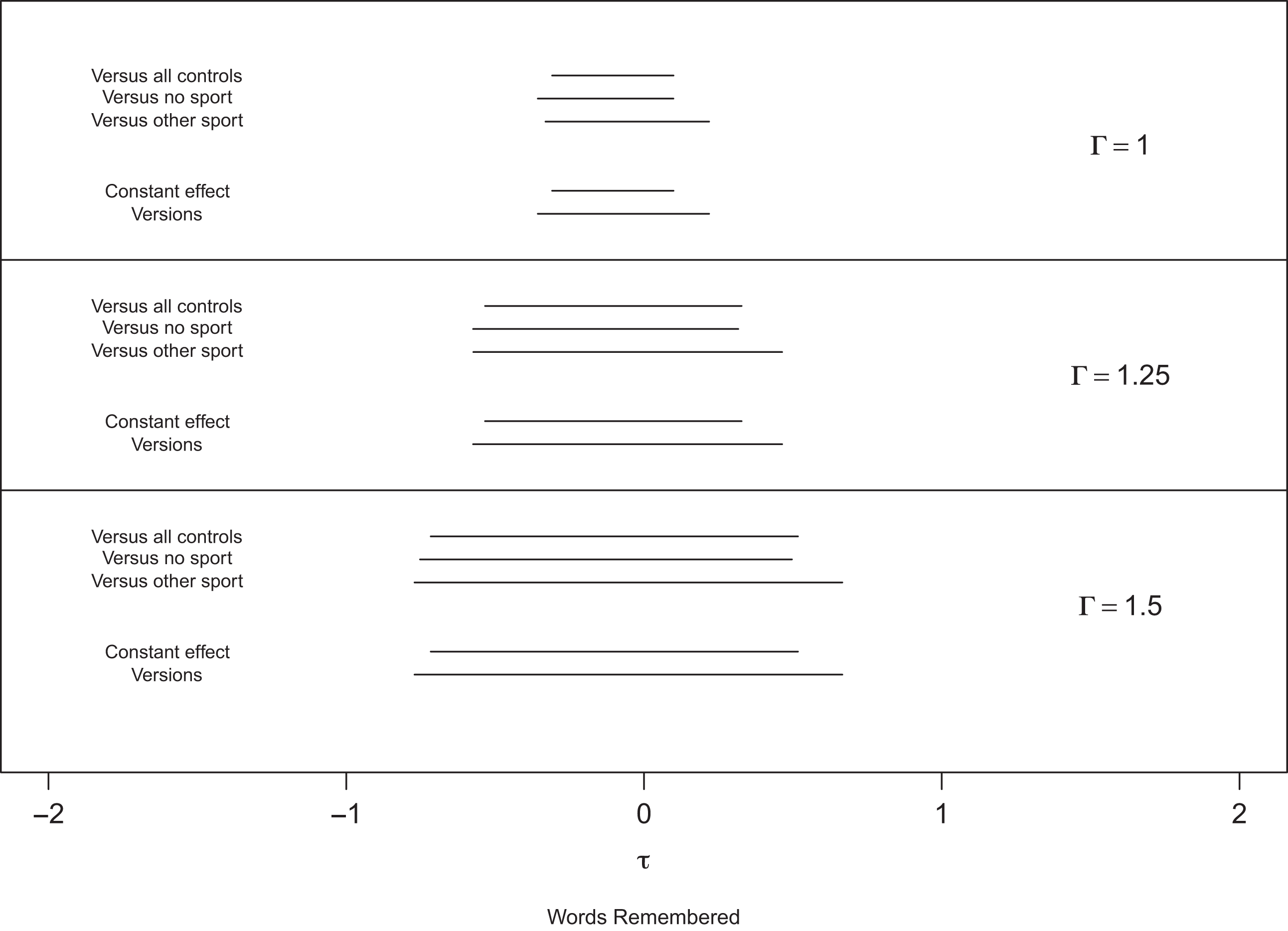
Comparison of interval estimates for the effect of high school football on the delayed word recall score. Note. The intervals for
In contrast, the intervals
6. Comparison to Conventional Approaches to Multiple Versions: F Tests and Bonferroni Correction
The method described in Subsection 5.2 makes an important trade-off: It prioritizes the primary comparison against all controls under the assumption of a constant treatment effect, allowing us to report the corresponding confidence interval with no correction, in exchange for the ability to distinguish between versions if they do, in fact, exists. In other words, our method emphasizes detection of nonzero, constant treatment effects over detecting different versions of the effect. Conventional approaches to multiple comparisons are often less focused and are designed to detect a broader range of departures from the null. For example, a simple Bonferroni correction places the primary comparison and the two versioned comparisons on equal footing. If the investigator does not suspect a priori that a particular alternative hypothesis is most likely, he may conduct an omnibus F test, whose power is distributed over a broad range of alternative hypotheses.
The researcher’s scientific aim should determine which method for multiple comparisons is most appropriate. With this guidance in mind, we compare our method to the omnibus F test and Bonferroni corrected intervals.
6.1. The Omnibus F Test
In exploratory analyses, the F test can be a useful “prelude to subsequent examinations of unplanned contrasts” (Steiger, 2004). However, in many studies, the researcher will have a particular contrast in mind. Several authors have argued that the omnibus hypothesis in analysis of variance studies be replaced with hypotheses that focus on a substantive research question, often involving just a single contrast (Rosenthal et al., 2000; Steiger, 2004). In the football study, we suspect a priori that versions are not terribly consequential and proceed first with our primary investigation of whether playing high school football accelerates the onset of cognitive decline. The hypotheses about versions are secondary to our main inquiry and are treated as such in our method.
The F test does not lend itself to effect size estimates, but we can compare it to our method by evaluating its power to reject Fisher’s sharp null hypothesis and the probability that
6.2. Bonferroni Corrected Intervals
In Figure 2, we compare the intervals returned by our version method to the three intervals returned by a Bonferroni correction (BC) to the comparison of the football players against all controls and each version of control. In the top panel, the BC interval using all controls is 22% longer than
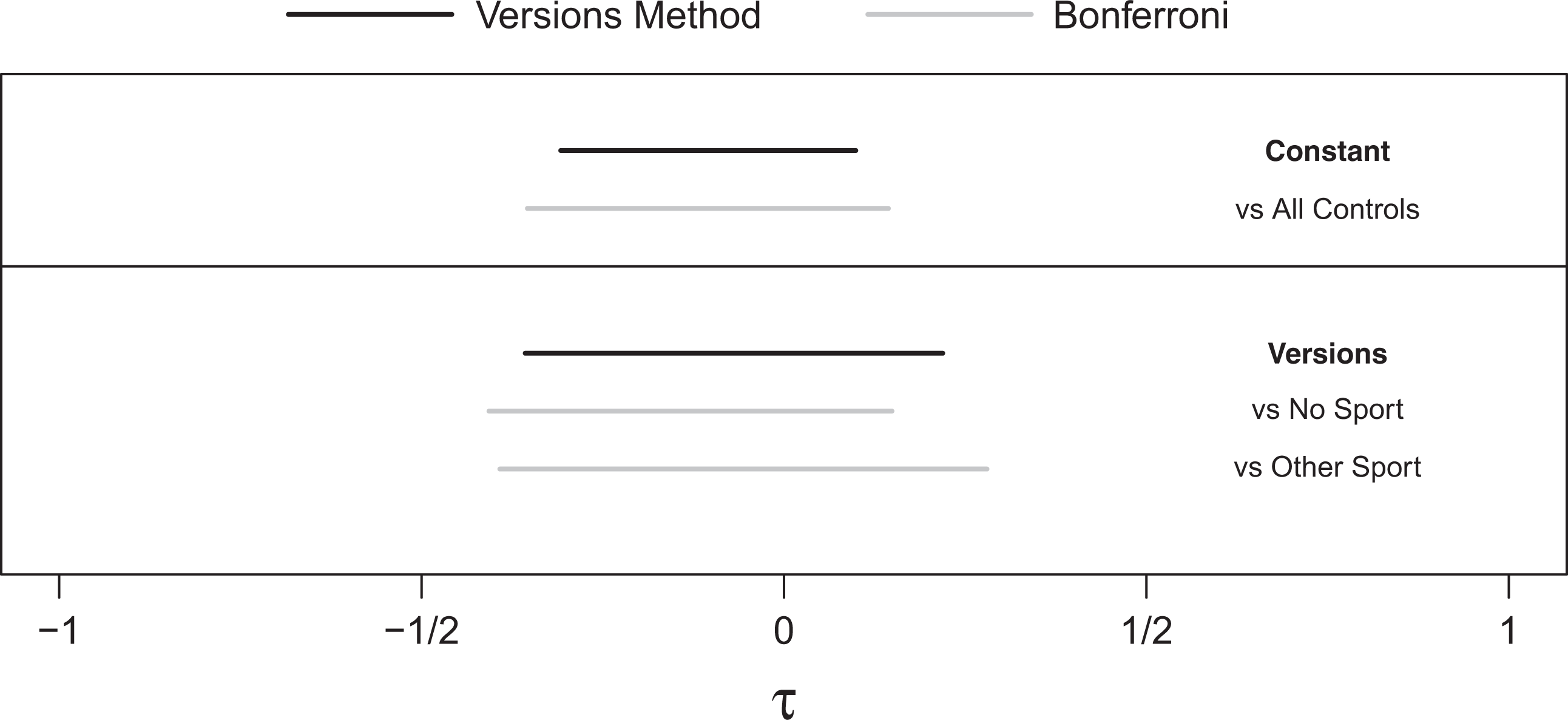
Comparison of
7. Versions, Effect Modification, and Insufficient Overlap
In the study of the effects of playing high school football on cognitive decline, the two versions of control and the football players have significant overlap in observed covariates. An anonymous reviewer suggested the following situation. Suppose that athletes who did not play football and nonathletes who did not play football differ noticeably on observed covariates such that a different set of football players were matched in the matchings using the different versions of control. If the treatment is heterogeneous, say it is modified by some observed covariate that differs between the two versions of control, does “this mean there are two versions of treatment or that there are two different groups of individuals that are involved in the two comparisons?” In this setting, the potential for treatment heterogeneity is aliased with the potential for versions of the treatment effect. But does this matter? The logic of Subsection 5.2 is agnostic to why there may be different treatment effects between versions. Thus,
8. Sensitivity to Departures From Random Assignment
So far, we have drawn inferences under the assumption that treatments are randomly assigned within matched sets. In an observational study, this assumption lacks support and is typically doubtful if not implausible. We examine sensitivity to bias from nonrandom assignment by assuming that two individuals with the same observed covariates may differ in their odds of treatment by at most a factor of
Aids to interpreting values of
Figure 1 shows the expansion of
In brief, there is no sign of an effect of high school football on memory scores. Could the absence of any sign of an effect reflect a substantial effect and bias in who plays football? To mask a true effect of
9. Discussion: Simultaneous Inference About One Question Under Different Assumptions
Investigators sometimes candidly report two or more statistical analyses valid under different assumptions. In the process, they often lose the several advantages of a single, simple, primary analysis, that is, a single analysis with high power against a nonzero constant effect because it uses everyone and avoids needed corrections for multiple testing when several statistical tests are performed. With less candor, investigators sometimes perform several analyses and report some but not all analyses, a perhaps common practice that no one would publicly advocate.
Versions of treatment arise in observational studies when treatment or control conditions found in available data may not be uniform, as they would be in a tightly controlled experiment. The investigator would like to follow the practice of clinical trials and report a single, primary analysis using everyone without multiplicity correction. Nonetheless, the investigator would like to speak to the possibility that there are versions of treatment or control conditions. The proposed method always reports two interval estimates. The first, shorter interval,
Appendix
Simulation Comparing the Power of the Omnibus F Test to
In this appendix, we compare the power of the omnibus F test to the power of our version method to detect departures from Fisher’s sharp null hypothesis under varying degrees of “versioning.” The results can be found in Table A1. When the degree of versioning is modest, the version method is more powerful than the F test.
Comparison of the Power of the Version Method (Columns 2 and 4) and the Power of the F Test (Columns 3 and 5) to Reject Fisher’s Sharp Null Hypothesis Under Alternative Hypotheses With Varying Degrees of “Versioning.”
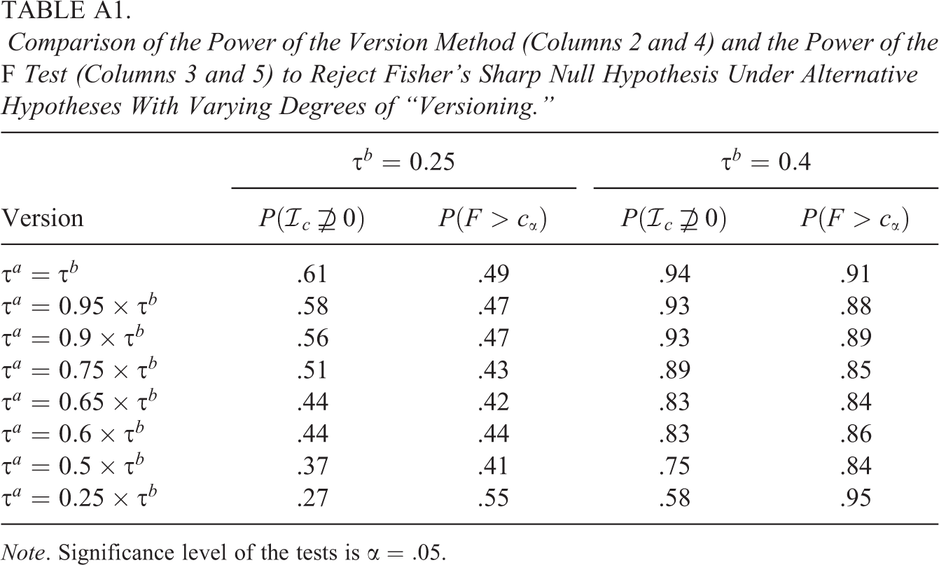
Note. Significance level of the tests is
Simulation Settings
Let there be
Footnotes
Declaration of Conflicting Interests
The author(s) declared no potential conflicts of interest with respect to the research, authorship, and/or publication of this article.
Funding
The author(s) received no financial support for the research, authorship, and/or publication of this article.