



Abstract
Cognitive diagnosis models (CDMs) are the statistical framework for cognitive diagnostic assessment in education and psychology. They generally assume that subjects’ latent attributes are dichotomous—mastery or nonmastery, which seems quite deterministic. As an alternative to dichotomous attribute mastery, attention is drawn to the use of a continuous attribute mastery format in recent literature. To obtain subjects’ finer-grained attribute mastery for more precise diagnosis and guidance, an equivalent but more explicit form of the partial-mastery-deterministic inputs, noisy “and” gate (DINA) model (termed continuous attribute profile [CAP]-DINA form) is proposed in this article. Its parameters estimation algorithm based on this form using Bayesian techniques with Markov chain Monte Carlo algorithm is also presented. Two simulation studies are conducted then to explore its parameter recovery and model misspecification, and the results demonstrate that the CAP-DINA form performs robustly with satisfactory efficiency in these two aspects. A real data study of the English test also indicates it has a better model fit than DINA.
1. Introduction
Cognitive diagnosis (CD) is a new trend in the development of contemporary psychometrics theory (von Davier & Lee, 2019). One of the main advantages of CD is that it can provide more in-depth and detailed diagnostic information to the subjects so that they can be provided with person-oriented remedial teaching and guidance for greater improvement (Leighton & Gierl, 2007; Rupp et al., 2010).
CD models (CDMs) are statistical models integrated with cognitive variables. They define the core structure of cognitive diagnostic assessment (CDA) and their properties directly determine the accuracy and effectiveness of CDA. The well-known CDMs developed in the last 20 years include the deterministic inputs, noisy “and” gate (DINA) model (Haertel, 1989; Junker & Sijtsma, 2001); the noisy inputs, deterministic, “and” gate (NIDA) model (Maris, 1999); the deterministic input, noisy “or” gate (DINO) model (Templin & Henson, 2006); the general diagnostic model (von Davier, 2008); and the generalized DINA (GDINA) model (de la Torre, 2011).
Most CDMs developed in the literature adopt discrete attribute mastery variables. That is, the subjects’ attribute mastery level is characterized by several discrete values. Initially, dichotomous values are used in CDMs (e.g., DINA, DINO, and NIDA) to characterize dichotomous attribute mastery level, with 0 representing nonmastery and 1 representing mastery (Chen et al., 2014; Cheng, 2009; Hsu et al., 2013; Mao & Xin, 2013; Wang, 2013; Wang et al., 2011). However, from a statistical point of view, it is deterministic to use only 0 and 1 to characterize the two levels of mastery (complete mastery or complete nonmastery; Zhan, Wang, et al., 2019). The framework of polytomous attributes was formed to alleviate the problem (Chen & de la Torre, 2013; de la Torre et al., 2010; Karelitz, 2004). But it did not solve the problem because the subjects’ diagnosis at each attribute level is still an absolute and unprecise value—0 or 1. In fact, the subjects’ attribute mastery level should not be deterministic because even for a group of subjects with the same value in a certain attribute (i.e., all of them are 0s or all of them are 1s), they still likely differ more or less in the attribute mastery degree. In such cases, it is that the differences in attribute mastery degree among subjects may be amplified or narrowed in a substantial level, resulting in less refined diagnosis and radically different guidance and remedies. In the CDMs, for example, the subject’s attribute profile is usually estimated via expected a posteriori (EAP), which is considered simplest, fastest, and conforms to the traditional Bayesian statistical thought (Huebner & Wang, 2011). During the process of estimation, the subject’s attribute mastery level is initially continuous and represented by attribute mastery probability (AMP) and finally just made an artificial discretization to facilitate CD. Suppose subjects A and B obtain a certain AMP of 0.4 and 0.6, respectively, in the estimation process. In that case, the diagnosis of their attribute mastery level will be truncated into 0 (complete nonmastery) and 1 (complete mastery), respectively, which amplify their difference, thus corresponding guidance and remedy will just be provided for A, but not for B. However, in fact, neither of them has a good attribute mastery level, and B also needs to consider whether guidance and remedy are necessary or not. Likewise, if their AMPs are 0.6 and 0.9, respectively, the problem still exists. Their difference will be narrowed, and A cannot get reasonable guidance and remedy. In addition, when partial mastery or incomplete mastery exists with subjects, the standard CDMs may not do a good job of explaining the heterogeneity in the responses (Shang et al., 2021). Therefore, it is reasonable to introduce continuous variables to describe the subjects’ attribute mastery degree in CDMs.
Earlier than the development of CDMs, the item response theory (IRT) was well established and widely used in educational and psychological application. It refers to a family of probabilistic models that attempt to explain the relationship between latent traits and their manifestations (Baker & Kim, 2004; DeMars, 2010; Embretson & Reise, 2000; Embretson & Steven, 2013; Hambleton & Swaminathan, 1985; Sijtsma & Junker, 2006; Van der Linden & Hambleton, 1997). In fact, multidimensional IRT (MIRT) models contain the idea of continuous latent traits and can also provide certain diagnostic information (Ackerman, 1994; Embretson & Yang, 2013; Reckase, 1997, 2009; Stout, 2007; Wang & Nydick, 2015; Whitely, 1980), and a typical one is the multicomponent MIRT model (Multicomponent latent trait models [MLTM]; Whitely, 1980). However, it should be noted that the latent trait θ in MIRT has no boundaries, and even if its absolute location is determined, its relative location cannot be determined, so MIRT cannot provide a direct and accurate diagnosis for subjects (Shang et al., 2021).
CDMs can also be assumed to be constructed in an unobservable multidimensional continuum to calibrate a subject’s location. Nevertheless, there is a major difference between them. Each attribute mastery (α) in CDMs now is in the range
Shang et al. (2021) propose several more specific and flexible CDMs-partial-mastery CDMs (PM-CDMs), which allow for partial mastery based on continuous attributes. They emphasized that these models are “mixed membership generations of the binary attribute CDMs.” However, the construction and estimation of these PM-CDMs are somehow complicated. As the DINA model is a simple and intuitive CDM, which can be easily estimated, a DINA-type form for continuous attribute profile (CAP), which is in fact an equivalent form of the PM-DINA model, is introduced in this article. To avoid confusion, it is referred to below as the CAP-DINA form. The CAP-DINA form is much simpler in terms of form, construction, and data-generating process of subjects, which gives better computation advantage.
The remainder of this article is structured as follows. In Section 2, the CAP-DINA form is proposed from a different perspective after reviewing the original DINA model; then, in Section 3, two simulation studies are presented. Study 1 simulates various conditions to explore the parameter recovery of the CAP-DINA form but with data-generating process of subjects different from the PM-DINA model, and the simulation in Study 2 compares the model misspecification of DINA and the CAP-DINA form. Section 4 applies the CAP-DINA form to English test data and demonstrates a good model fit. Finally, this article is concluded with a discussion and some directions for further research.
2. The CAP-DINA Form
2.1. The DINA Model
The DINA model is a simple, intuitive parameterized model that is easily estimated and has received much attention in recent CDM literature. As a result, we will take DINA as an example in this study. We assume the number of attributes measured by the test is K. The item response function (IRF) for the DINA model, which represents the correct response probability of Subject i on item j, is defined as follows:

in which

where
2.2. Formulation of CAP-DINA Form
Subjects’ attribute mastery in standard CDMs is dichotomous—mastery or nonmastery, which is deterministic. In addition, from a statistical point of view, a subject’s attribute mastery degree is usually determined by calculating the proportion of their correct response on that attribute. The greater the proportion, the higher the attribute mastery degree. As a result, it is reasonable to assume the attribute mastery degree to be continuous. In this article, we assume Subject i’s attribute mastery

in which

An example of its IRF computation is given as follows:
if


2.2.1. Monotonically increasing property
For any fixed Item j, the larger the subject’s mastery proportion (
Taking the first derivative of Equation 3 with respect to

Considering the monotonicity restriction

So,

that is,

As a result, the CAP-DINA form satisfies the monotonically increasing property with respect to
2.2.2. Relationships with DINA
The core difference between the CAP-DINA form and DINA is that the former assumes each subject has a CAP
2.2.3. Relationships with MLTM
In MIRT, there is a typical model-MLTM (Whitely, 1980) similar to the CAP-DINA form. They have in common that they both are noncompensatory diagnosis models based on the products of the continuous latent traits. The differences between them are as follows: (1) The latent trait
2.2.4. Relationships with PM-DINA
Four similarities can be found between the CAP-DINA form and the PM-DINA model (Shang et al., 2021): (1) They both have the assumption that each subject has a continuous attribute mastery on the interval
Shang et al. (2021) allow that the subject’s attribute mastery is also partial and continuous on the hypercube
For DINA model, the ideal response

which can also be represented as

Then, the probability of a positive response to Item j


For a subject with a general mastery score

in which
Next, we simplify Equation 13.
The number of all the possible attribute profiles
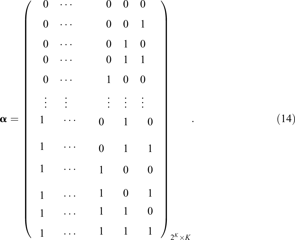
The rows of (i) Without loss of generality, suppose that Item j measures the first

For
in which
It can be expressed as

Note that each value in the first m columns is 1.
Because the number of
According to Equation 11,


Combining Equations 13, 16, and 17, we can get

Note that

First, we calculate
For

Here, according to Equation 12,




⋮

As we can see, the first left-hand side of Equations 21 through 25 is the same. Because
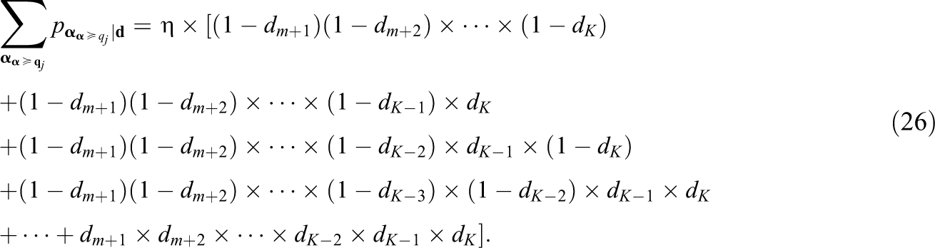
To calculate Equation 26, we just need to calculate the part in the square bracket first.
To simplify the part in in the square bracket, we think of the
So, the sum of the part in the square bracket of Equation 26 is also 1, then

Hence, the first part in Equation 18

Second, we calculate
According to Equation 19,

then

Substitute Equations 29 and 30 into Equation 18,

The above is the proof for Item j measuring the first (ii)If the
So, the IRF in the CAP-DINA form is essentially equivalent to the IRF in the PM-DINA model.
2.2.5. Model identifiability
The model identifiability issue is critical in Bayesian approach. Shang et al. (2021) represent the PM-DINA model by a restricted class model (RLCM), which is identifiable if the Q-matrix satisfies certain structural conditions (Gu & Xu, 2020; Xu, 2017). With this equivalent RLCM representation, the identifiability of the model parameters of PM-DINA is expected to be established under a similar set of structural conditions for the Q-matrix (Shang et al., 2021). Since the CAP-DINA form is shown to be essentially equivalent to the PM-DINA model, we would also conclude that the identifiability of CAP-DINA form could be established if the Q-matrix satisfies the similar structural conditions.
2.3. Model Estimation
The parameters of the CAP-DINA form are estimated via the Bayesian technique using the Markov chain Monte Carlo (MCMC) algorithm, which is implemented in the freeware JAGS programme (Version 4.3.0; Plummer, 2015). By default, the Gibbs sampling algorithm is used by JAGS (Gelfand & Smith, 1990), and an additional tutorial on using JAGS for Bayesian CDM is provided in Zhan, Jiao, et al. (2019).

where
The hyperpriors of

The hyperpriors of

where
The response of Subject i to Item j is assumed to be independently distributed following a Bernoulli distribution:

where
The priors of item parameters sj and gj is specified as follows:


in which T is a truncation function and
Finally, the posterior mean is treated as the estimate value for the item parameters (i.e., sj
and gj
), and the posterior mode is treated as the estimate for the person parameters (i.e.,
It is necessary to compare the data-generating processes of a subject between the CAP-DINA form and the PM-CDM model as they will affect the recovery of the values of the parameters. In order to understand the difference more intuitively, we illustrate it with Figure 1. The PM-CDM model introduces for each subject a vector of dichotomous auxiliary latent indicators
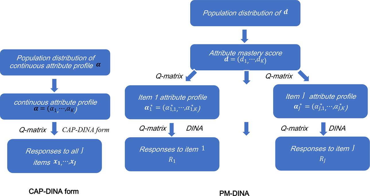
Continuous attribute profile-deterministic inputs, noisy “and” gate (DINA) form and partial-mastery-DINA date-generating processes for a subject.
3. Simulation Studies
Two simulation studies were conducted to explore the performance of the CAP-DINA form under various conditions. Specifically, Simulation Study 1 was to demonstrate the model parameter recovery accuracy. The data were simulated from the CAP-DINA form and analyzed with the true model. Simulation Study 2 was to compare the misspecification of the CAP-DINA form and the DINA model. Specifically, both the DINA model and the CAP-DINA form are fitted for the DINA and the CAP-DINA form generated datasets.
3.1. Simulation Study 1
3.1.1. Design and data generation
Two numbers of independent attributes (

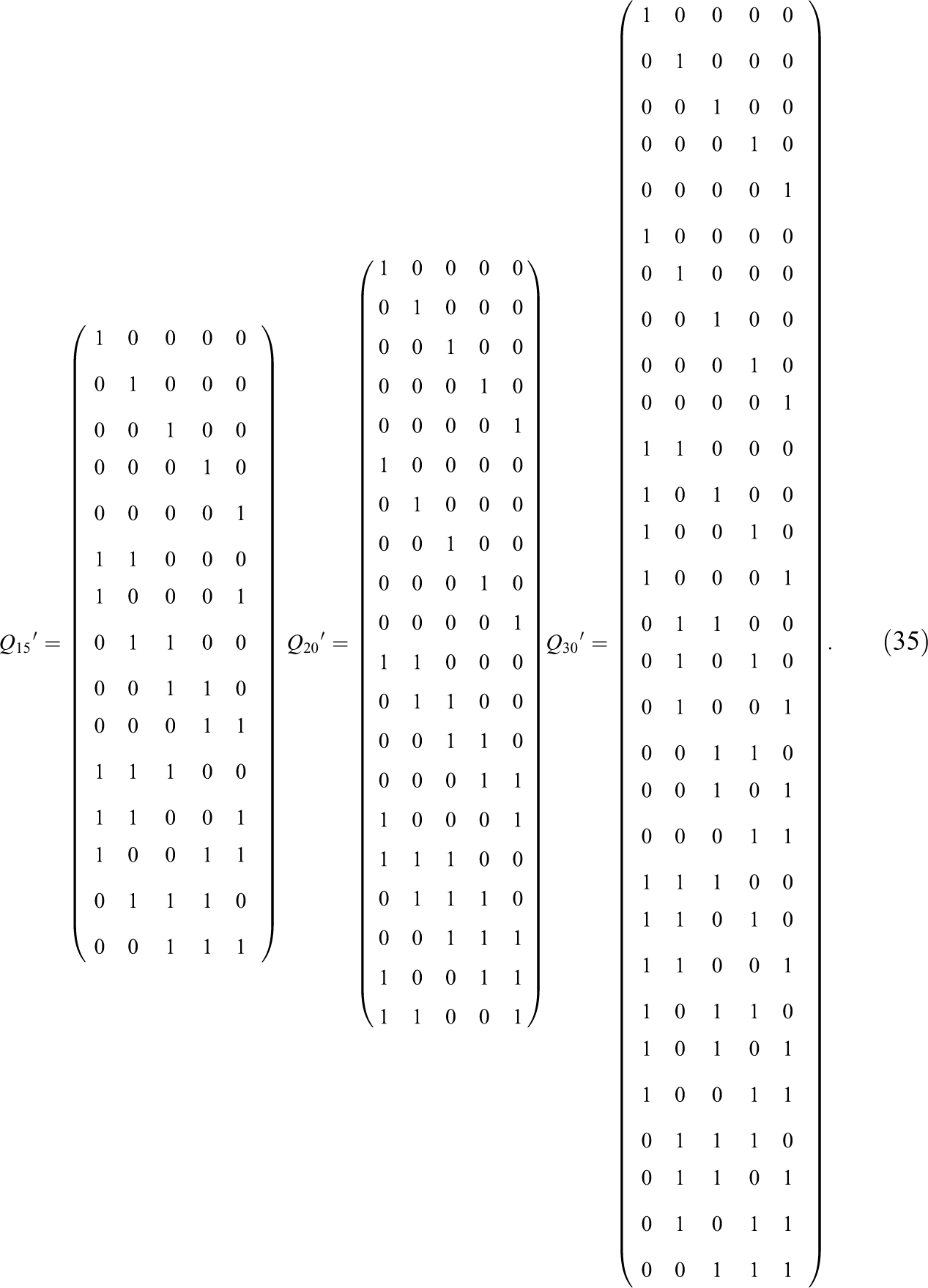
3.1.2. Analysis
The CAP-DINA form was fitted to each replication. For each replication, two Markov chains with random starting values were used and each chain had 5,000 iterations, with the first the numbers of 2,000 iterations in each chain as burn-in, and the remaining 3,000 iterations for model parameter inference. The potential scale reduction factor
To evaluate parameter recovery accuracy, for the item parameters, the absolute bias standard error (ABSE) and the root mean square error (RMSE) averaged across all items and overall replications were both reported; for the person parameters, ABSE and RMSE of each attribute averaged across all subjects and overall replications were both reported.
3.1.3. Results
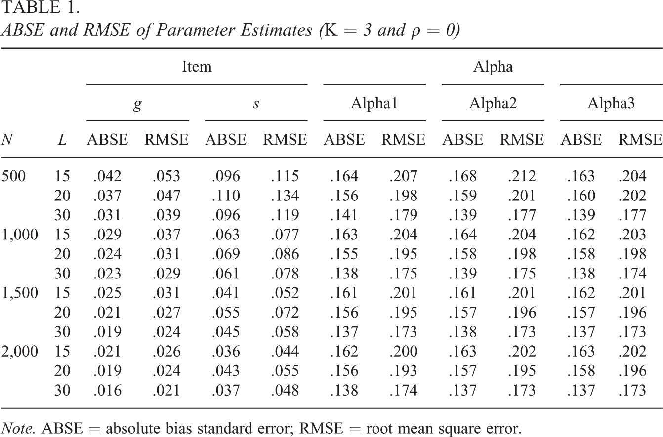
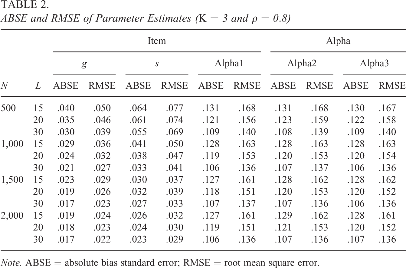
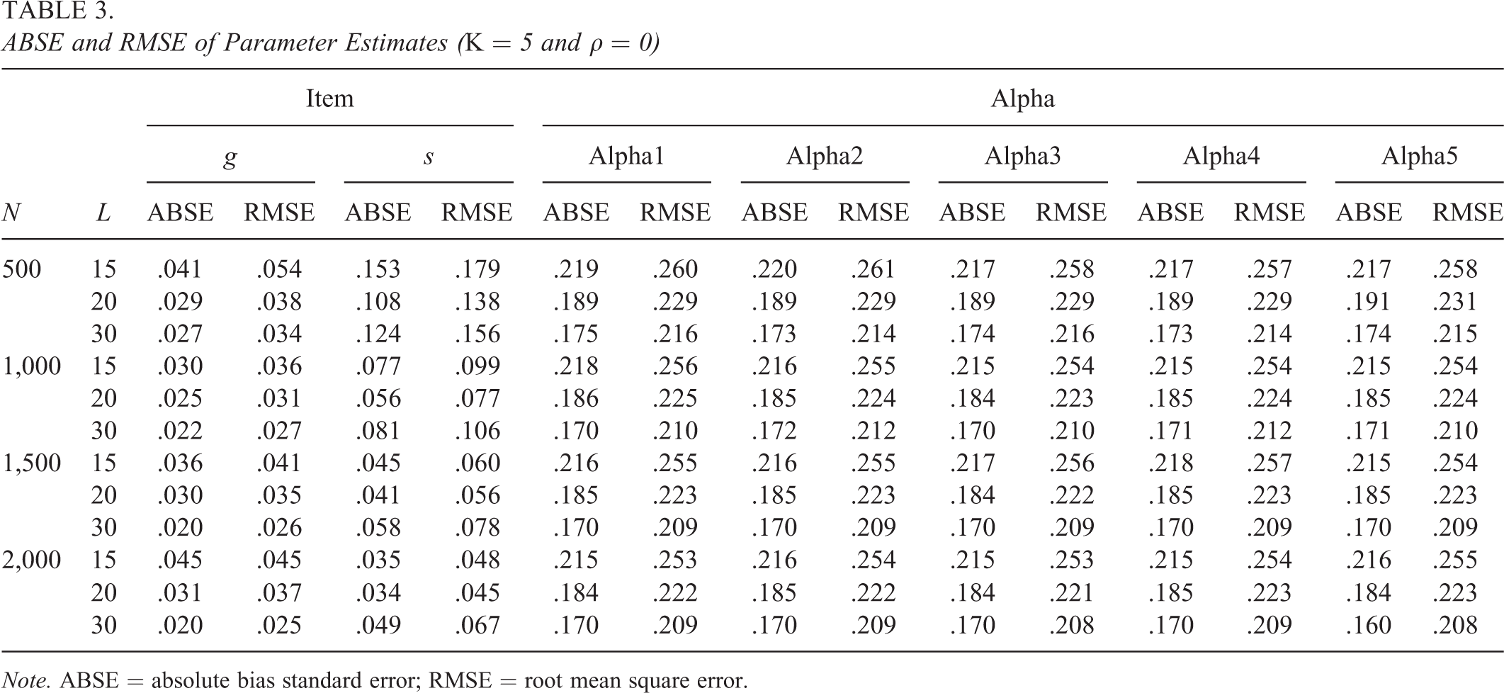
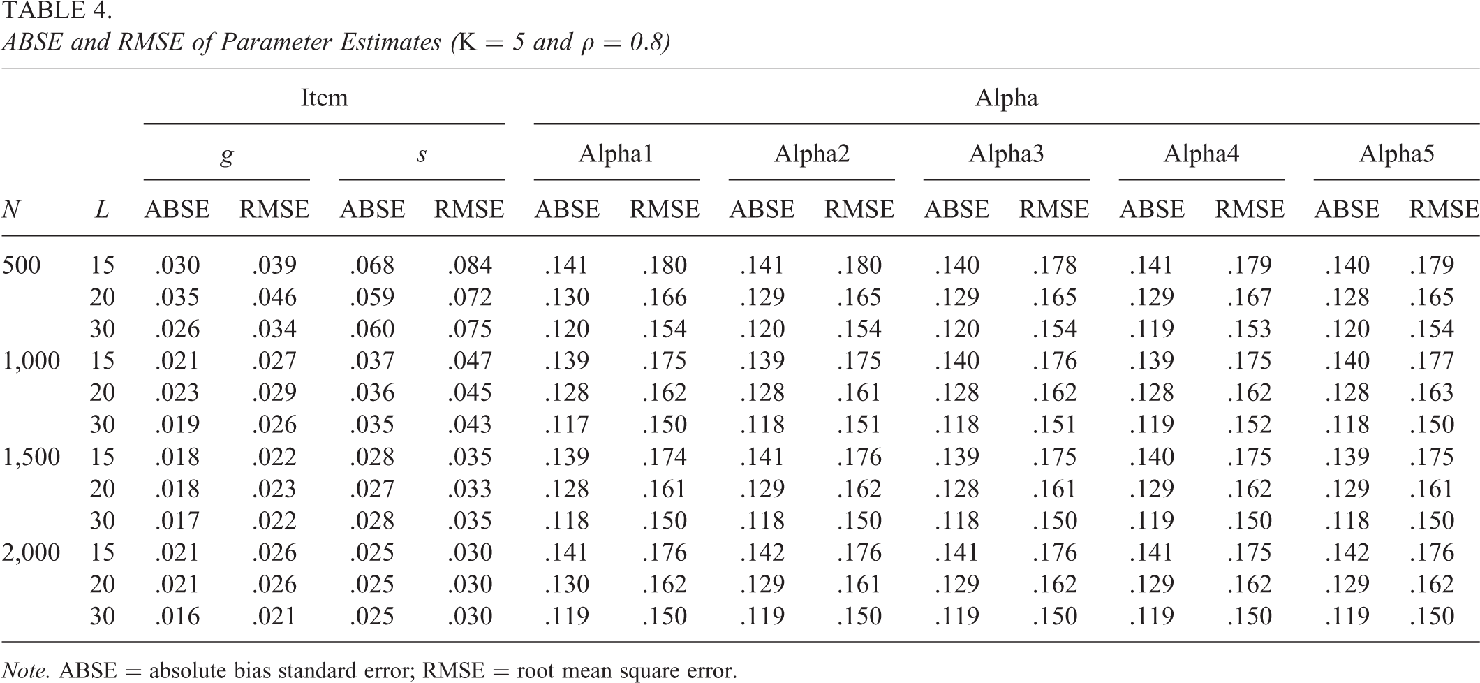
Tables 1 through 4 present the ABSE and RMSE of parameter estimates in various settings, respectively. We start by analyzing each table individually, and several conclusions can be drawn. We take Table 2 as an example for specific analysis. First, for a test given a fixed length (L), the larger the sample size (N), the smaller the ABSE and RMSE. For example, for
ABSE and RMSE of Parameter Estimates (K = 3 and
Note. ABSE = absolute bias standard error; RMSE = root mean square error.
ABSE and RMSE of Parameter Estimates (K = 3 and
Note. ABSE = absolute bias standard error; RMSE = root mean square error.
ABSE and RMSE of Parameter Estimates (K = 5 and
Note. ABSE = absolute bias standard error; RMSE = root mean square error.
ABSE and RMSE of Parameter Estimates (K = 5 and
Note. ABSE = absolute bias standard error; RMSE = root mean square error.
Next, we compare Tables 1 through 4. First, comparing Tables 1 and 3, it can be seen that with the same sample size and test length, the larger the K, the larger the ABSE and RMSE for person parameter estimates, that is, the less precise the person parameter estimates, which is also expected since fixed items provide fixed information on more person parameter estimation, which indicates with the same size of data information, the more parameters to be estimated as the attribute number increases, the less precision for estimation. This also can be seen from the comparison of Tables 2 and 4. Second, comparing Tables 1 and 2, it can be seen that both item and person parameters have better estimation accuracy when the correlation coefficient ρ is 0.8 than
In general, the MCMC estimation method demonstrates a good parameter recovery in this study.
3.2. Simulation Study 2
3.2.1. Design and data generation
The Q-matrices, mean vector
3.2.2. Analysis
For the MCMC estimation of CAP-DINA form, the number of chains, burn-in iterations, and post-burn-in iterations were set the same as those in Simulation Study 1. For DINA model, the EAP method was used for estimation. Certain indicators were used to evaluate the two models. Specifically, (1) when the true model was DINA, that was, the data were generated following DINA, we evaluated the two models by total ABSE and RMSE of item parameters instead of each item parameter and attribute marginal match ratio (AMMR), that is,
3.2.3. Results
Tables 5 and 6 present the results for all the 16 settings. We take Table 5 as an example for specific analysis. Table 5 reports the results of the condition (
Results of Simulation 2 for K = 3 With N = 500
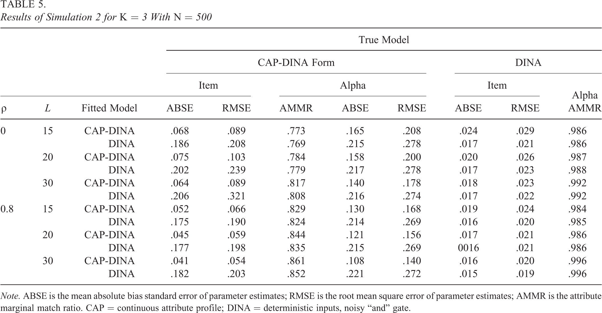
Note. ABSE is the mean absolute bias standard error of parameter estimates; RMSE is the root mean square error of parameter estimates; AMMR is the attribute marginal match ratio. CAP = continuous attribute profile; DINA = deterministic inputs, noisy “and” gate.
Results of Simulation 2 for K = 5 With N = 1,000
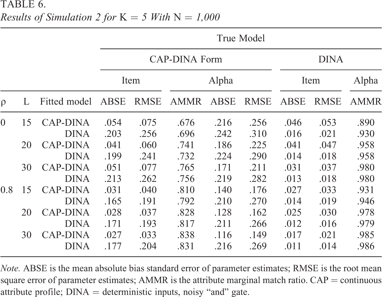
Note. ABSE is the mean absolute bias standard error of parameter estimates; RMSE is the root mean square error of parameter estimates; AMMR is the attribute marginal match ratio. CAP = continuous attribute profile; DINA = deterministic inputs, noisy “and” gate.
4. Real Date Examples
To illustrate the application of the CAP-DINA form, we apply both the CAP-DINA form and the DINA model to the English tests dataset collected by the Examination for the Certificate of Proficiency in English and introduced within the CDM package in R software, which was analyzed in some previous studies, containing responses to 28 items designed to assess three skills—morphosyntactic form (
The Q-matrix and MCMC estimates of the posterior item parameters based on CAP-DINA form are reported in Table 7. First, the 28 items display variability in estimated item parameters gj
and sj
. Specifically, gj
ranges from 0.019 to 0.782 and sj
ranges from 0.013 to 0.032, that is,
Q-Matrix for English Test Data and the Estimation Results

Table 8 reports AIC, BIC, and DIC (Spiegelhalter et al., 2002) comparison between the CAP-DINA form and the DINA to assess the relative model fit. This demonstrates a better model fit than DINA due to its small AIC, BIC, and DIC.
AIC, BIC, and DIC for English Test Data
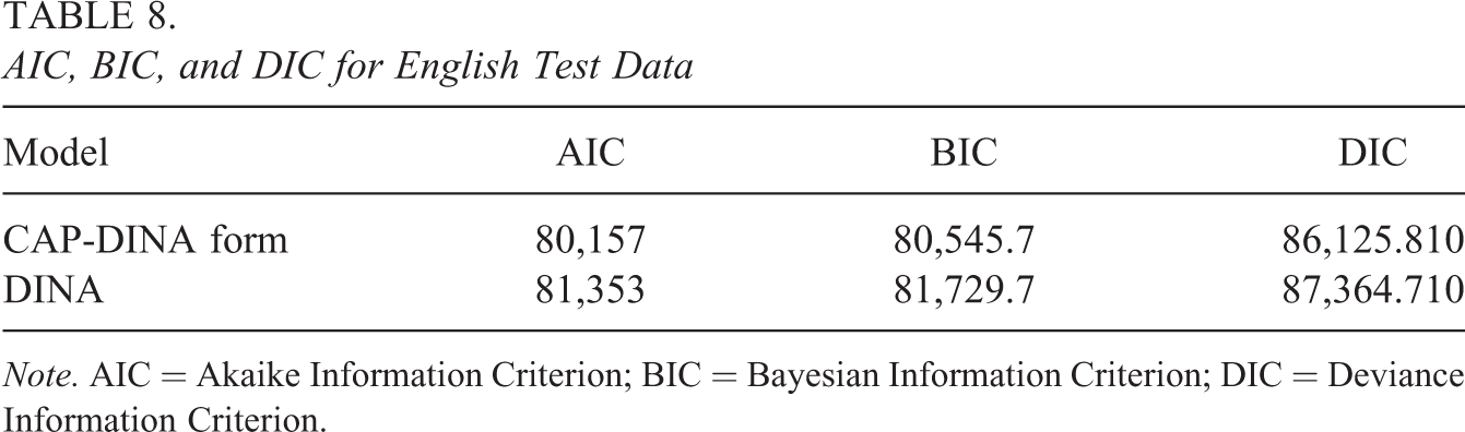
Note. AIC = Akaike Information Criterion; BIC = Bayesian Information Criterion; DIC = Deviance Information Criterion.
5. Conclusion and Discussion
In order to obtain more precise and in-depth diagnostic information about subjects’ attribute profiles instead of only mastery or nonmastery, we propose a flexible DINA for CAP-DINA form-an equivalent form of the PM-DINA model, which subsumes DINA model as a special case. A Bayesian technique with MCMC algorithm is developed with accurate parameter recovery in Simulation Study 1. Simulation Study 2 compares the model misspecification of DINA with the CAP-DINA form and the CAP-DINA form performs more robust. Specifically, when the data are generated under continuous attribute condition, the CAP-DINA form fits the simulated data better than DINA model, and when the data are generated under binary attribute condition, the results of the CAP-DINA form are comparable to that of DINA model. The real data study demonstrates the application of CAP-DINA form in practical educational testing and shows that CAP-DINA form has a better fit than DINA in English test data through the goodness-of-fit measures, such as AIC, BIC, and DIC. Therefore, it is believed that the CAP-DINA form has more advantages than DINA and could be widely accepted in application.
The simulation and the real data studies also show that (1) the CAP-DINA form has the advantage over MIRT models, for the former can determine subjects’ relative location and then provide a direct and accurate diagnosis for subjects. With a simple form, the CAP-DINA form also overcomes the limitations of noncompensatory MIRT models; (2) although the CAP-DINA form is a CCM like the CCM, the CCM only contains person parameters but no item parameters; thus, the stochastic components are absorbed into the subjects’ ability profiles, while the CAP-DINA form adds item parameters; thus, part of stochastic components are absorbed into the items. In this regard, the CAP-DINA form is more reasonable; and (3) both the CAP-DINA form and PM-DINA model assume CAP and are essentially equivalent in terms of IRF. However, model complexity of PM-DINA leads to high computation cost especially when the number of attributes is large (Shang et al., 2021), whereas the estimation within CAP-DINA form is relatively straightforward and efficient due to its simplicity in terms of form, construction, and data-generating process of subjects. In conclusion, the concept of attribute continuation and the proposal of CAP-DINA form are considered significant, with the anticipation that it opens a new research area for CDM.
With the CAP-DINA form, a potentially promising application procedures related to Fisher information (FI) could be developed using the continuity feature of the attribute mastery. FI has been developed and widely used in IRT models (Chang & Ying, 1996). Although the distance information such as Shannon entropy and Kullback–Leibler Divergence (Claude Shannon, 1948; Cover & Thomas, 1991; Kullback, 1959) are also applied, FI has its own unique function that it reflects the precision of the parameter estimation by measuring each subject’s estimation error. However, the methodological and theoretical developments of FI in CDM appear to lag behind due to the discreteness of attribute profile. The introduction of attribute continuity in CAP-DINA form makes it possible to propose Fisher-type information in CDM. Hence, the model will have more applications based on Fisher-type information.
Another interesting extension of this study is to nest the continuous attribute into polytomous attribute CDMs (Chen and de la Torre, 2013; von Davier, 2008). Although the framework of polytomous attributes has been put forward to relax the binary assumption of attributes so as to provide a more accurate diagnosis for subjects, but the diagnosis at each attribute level of is still an absolute and unprecise value—0 or 1. The idea of attribute continuity would be a solution, which allows us to construct continuous polytomous attribute CDMs, such as polytomous CAP-DINA form.
Extending other CDMs by incorporating the idea of attribute mastery continuation will also be interesting. Due to the simplicity and intuitiveness of DINA, the attribute mastery continuation is just applied in the DINA model in this article. In fact, there are varieties of CDMs, such as GDINA (de la Torre, 2011) and RRUM (Hartz, 2002), each with different roles. Similar continuation could be applied on other CDMs. The direct extension can be DINO (Templin & Henson, 2006), because the DINA and the DINO models share a “dual” relation (Ko¨hn & Chiu, 2016). How to extend the idea to more CDMs is an interesting topic.
Although the real date study indicates the CAP-DINA form has a better fit than DINA in English test data, the following two issues should be noted, (1) the heterogeneity of item complexity and attribute difficulty may result in the heterogeneity of item parameters, so the item complexity and attribute difficulty is worth studying in the future; and (2) large estimates of gj and sj , especially gj , may be related to the misspecification of Q matrix. Consequently, it is necessary to conduct additional research of the item quality of the English test (Yu & Cheng, 2020).
Finally, although the MCMC algorithm is developed for CAP-DINA form estimation and provides accurate parameter recovery, the estimation process is somehow time-consuming, and the computation efficiency needs to be improved further. In particular, there are situations where efficiency is necessary, such as computerized adaptive test, and the development of an efficient algorithm for CAP-DINA form is imperative. It is known that the EM algorithm is much faster than MCMC. To develop a more efficient EM-type algorithm for the CAP-DINA form would be our future research direction.
Footnotes
Declaration of Conflicting Interests
The author(s) declared no potential conflicts of interest with respect to the research, authorship, and/or publication of this article.
Funding
The author(s) disclosed receipt of the following financial support for the research and/or authorship of this article: This study is supported in part by the 14th Five-Year Plan for Education Science in Jiangxi Province (Grant No. 21YB257, 21YB027), the 14th Five-Year Plan for Social Science in Jiangxi Province (Grant No. 21JY06, 22JY16), and the Humanities and Social Sciences Program of Jiangxi Provincial Department of Education (Grant No. XL20202).
