On the profitability and errors of predicted prices from deep learning via program trading

Abstract

Researches on using deep learning models to predict prices usually take magnitude-based error measurements (such as $R^{2}$ ) to measure the quality of learning models. Whether the forecasted prices for the models with the lowest error measurement can produce the most profit in actual trading is an issue with little research.

In this study, we first find the parameter sets of LSTM and TCN models with low magnitude-based error and then use program trading to find out their profitability. The relationships between these profitability and error measurements are analyzed and studied on three commodities: gold, soybean, and crude oil (from GLOBEX).

Our findings are: with given parameter sets, if merchandise (gold and soybean) is of low averaged magnitude error, then its profitability is more stable. If it is of a more significant magnitude error (crude oil), then its profitability is unstable. A high positive correlation does not exist between the profitability and error measurement, and TCN outperforms LSTM in almost all our examples.

Our research indicates that, in assessing the performance of deep learning, how to use the predicted values in applications and the application results could also be part of the quality measurement for the model assessment in the learning.

Keywords

Deep learning price prediction program trading time sequence LSTM TCN

1. Introduction

Forecasting future values of time series is the subject of research [1, 2, 3]. Deep learning provides better results for the prediction than linear models [1, 4]. Yet, few works offer guidelines on how to apply the forecasted values in actual trading, as well as whether the predicted values with lower error measurement (such as $R^{2}$ and MSE) can offer better trading profitability.

Different merchandise may need different deep learning models. LSTM is suitable for merchandise with lower volatility [1, 5], and TCN may perform better on merchandise with higher volatility due to its pre-filtered local patterns [6]. Finding proper deep learning models and parameter sets for the commodities is the first step in studying their profitability.

Program trading can systematically and repeatedly explore the profitability of the target learning models. The utilized trading program should match the timing when target learning models generate predicted prices to reduce unnecessary logical errors, such as using unavailable future data in testing.

We explore the related works in Section 2. In Section 3, a three-stage process is proposed to evaluate errors in deep learning models with the trading program for assessing the profitability of predicted prices. Section 4 details the results of the experiments on three commodities. The conclusion comes in Section 5.

2. Related works

2.1 Time series

Variables inherently ordered by time are called time series, such as a stock or currency prices. They are usually not expressible as a linear function since the volatility and fluctuation may change as time progresses. With the right data mining technology and long enough data, a self-adaptive learning model may provide good prediction [7]. Deep learning models are one of this kind.

2.2 Neural networks as learning models

Neural networks use layers of neurons with adjustable weights to capture the non-linear relationship between input and production [8]. The neurons mimic the human brain to work as simple units, which are highly connected. Weights on the links may substantially affect the networks, and the overfitting problem occurs. The number of layers, the numbers of neurons in each layer, and parameters such as the dropout rate should be regulated to avoid the overfitting problem when utilizing the models.

2.3 Deep learning

In traditional data mining, features are usually manually specified by experts in advance, and this is called feature engineering. For data with inherently complex features, feature engineering is hard. Deep learning is a multi-layered neural network with sophisticated routing between both the interconnected neurons and layers. Deep learning has the effects of automatic feature engineering through those layers of neurons [8]. However, the quality of deep learning is profoundly affected by its training process. For example, the gradient should be managed appropriately to avoid gradient exploding or gradient vanishing problems.

2.3.1 Deep learning for time series

With cross-layered connectivity, recurrent neural network (RNN) accomplishes deep learning on time series [8]. By redirecting the output value back to the input, RNN acquires the “memory” effect. Nevertheless, its uncontrolled utilization of memory may lead to more noise. LSTM (Long-Short Term Memory) maintains the memory effect of RNN but keeps only the important one for future use. Pant [1] successfully applies LSTM to predict the currency fluctuation of the US dollar and the Russian Ruble.

CNN (Convolution Neural Networks) excels at image recognition but performs less robust in time series prediction. Bai [9] proposes TCN (Temporal Convolutional Networks) for time-series prediction and get better results than LSTM in many situations. TCN, similar to CNN, acquires signals simultaneously, where RNN acquires signals sequentially. TCN regulates the sliding windows of convolution to achieve the time series prediction. Thus, in this paper, TCN is also explored, in addition to LSTM.

2.3.2 Activation functions

In neural networks, the activation function ensures the input and output are not linearly related since the linear relationship between input and output significantly reduces the expressiveness of the networks. Commonly used non-linear functions are Sigmoid, tanh, and ReLu [10]. Sigmoid is best for classification problems as it maps inputs to values between 0 and 1. Tanh and ReLu are for non-classification problems where ReLu speeds up the training and avoids the gradient vanishing problem [11]. Hochreiter [12] provides another activation function, SeLu, for time series problems. SeLu can converge well, avoid gradient exploding or vanishing problems, and also perform well in deeper layered networks. Thus, we test both SeLu and ReLu in our TCN experiments. However, due to the limitation of Cudnn in our LSTM model, only Tanh can be used as the activation function in our LSTM experiments. For convenience, the definition of SeLu from [12] is listed here:

$\displaystyle\textit{SeLu}:\textit{SeLu}\left(x\right)=\lambda\left\{{{\begin{% array}[]{ll}x&\text{if }x>0\\ \alpha e^{x}-\alpha&\text{if }x\leqslant 0\\ \end{array}}}\right.$ (1)

2.3.3 Loss function

The loss function measures the difference between the predicted and actual values where absolute or squared distance may be the measurements. This distance also indicates regression errors. Minimizing loss function improves the quality of regression. Two commonly used loss functions, MAE and MSE, are shown as follows:

$\displaystyle\textit{MAE}:\frac{1}{n}\sum_{i=1}^{n}\left|{y_{i}-\hat{y}_{i}}\right|$ (2) $\displaystyle\textit{MSE}:\frac{1}{n}\sum_{i=1}^{n}\left({y_{i}-\hat{y}_{i}}% \right)^{2}$ (3)

MAE tends to find a local optimum when the gradient increases. MSE could be affected by outliers, and normalization can ease the problem. Thus, MSE is more popular than MAE [13].

2.4 Measuring the quality of deep learning models

MSE or coefficient of determination ( $R^{2}$ ) is used in deep learning to measure the quality of the learning. $R^{2}$ is developed from MSE with variance as the denominator to ensure its values always range between 0 and 1, which allows comparisons across different features. Its function is as follows:

$\displaystyle R^{2}\left({y,\hat{y}}\right)=1-\frac{\sum\left({y_{i}-\hat{y}_{% i}}\right)^{2}}{\sum\left({y_{i}-\hat{y}}\right)^{2}}$ (4)

When the number of samples increases, $R^{2}$ may lose accuracy as its numerator increases un-proportionally. Hyndman [14] suggested the use of MASE to reduce the problem. MASE uses the naïve projection of in-sample data as the denominator to reduce the errors from out-sample data and provides better normalization. Its function is as follows:

$\displaystyle\textit{MASE}=\textit{mean}\left({\left|{q_{t}}\right|}\right)$ (5) $\displaystyle q_{t}=\frac{e_{t}}{\frac{1}{n-1}\sum_{i=2}^{n}\left|{x_{i}-x_{i-% 1}}\right|}$ (6) $\displaystyle e_{t}=\left|{y-\hat{y}}\right|$ (7)

2.5 Program trading

Program trading uses a set of rules expressed as programs to buy and short merchandise. It can apply to merchandise with historical price data repeatedly to verify that the provided rules are indeed profitable [15]. We use Multicharts [16] in this research due to its broad user base and easy readability.

2.6 Predicted prices and trading profitability

Quality of the predicted prices from machine learning techniques (including deep learning) and how the predicted prices lead to trading profitability are, in fact, two different issues.

The quality of the predicted prices measures the difference between the actual value and predicted value where MSE, MAE, MASE, and coefficient of determination ( $R^{2}$ ) are the commonly used measures [13, 14]. Previous works, such as works on predicting currency [1] stock indexes [3] and stock prices [6], measure their improvement using these criteria.

In addition to the quality of predicted value, how we use the predicted prices during the trading decision (e.g., buy, short, or liquidate the positions), usually called “trading strategy,” also determines the trading profitability significantly. A trading strategy can be better studied using program trading [15, 16]. Net profit, maximum drawdown, and annual growth rate are commonly used to measure the quality of a trading strategy [17]. Works in [1] used a simplified trading strategy with only net profit listed, and works in [1, 3] do not show trading results.

For completeness, measurements considering both the quality of predicted prices and trading profitability are compared and analyzed in our works.

3. System design and implementation

Our proposed system design and experiments are divided into three stages, as expressed in Fig. 1. The first stage focuses on finding better models and settings from LSTM and TCN based on traditional error measurements: $R^{2}$ and MASE. In the second stage, the predicted values from the chosen models are used in the trading program to compute their profitability and error measurement. In the third stage, all aforementioned experimental results are compared to study their relationships and find potential hidden rules.

Figure 1.

Three-staged system design and experiments.

3.1 Predicting next-day’s close prices and corresponding trading programs

Most works on deep learning models address their contribution by measuring the improvement based on $R^{2}$ for their proposed models. However, our research further addresses the trading profitability of predicted values as another quality measurement. The used trading model should match the timing where the next-day predicted price is available, and this model should be simple enough without adding other factors to dilute the profitable effect of the predicted next-day value.

As shown in Fig. 2, we propose to enter the market five minutes before the close of today and liquidate the position before the end of the next trading day. A buy position is opened when the predicted close price for the next day is proportionally higher than today’s close price. A percentage-based stop-loss is used to liquidate the position if the position suffers certain percentage of loss in the coming trading day. The optimization mechanism of program trading will find the exact percentages for entry and stop-loss [17]. The exact opposite rules apply to the short position. If this simple trading program can profit, we can attribute most of the success to the precision of the anticipated next-day close value.

In existing researches, today’s close price is always used to predict the next-day close price [1, 4]. However, when today’s close price is available for the prediction, the market is already closed for trading. To avoid this problem, we use the price five minutes before the close as the actual input to predict the next-day close price of the proposed trading program. For the feasibility of this modification, we further analyze the fluctuation of the last five minutes before the market close for our studied merchandise. The average price fluctuation for these merchandise in the last five minutes is less than 0.01%, as shown in Table 1. We further use the actual close price and the price five minutes before the market close as two different inputs for the same LSTM models. The goal is to know how different the predicted next-day values are from the actual next-day close. As shown in Table 2, the $R^{2}$ for these two different inputs are almost the same.

Table 1
Price difference between today’s close and five minutes before the close

	Soybean	Crude oil	Gold
Average	0.075 (0.007%)	0.002 (0.003%)	$-$ 0.023 ( $-$ 0.002%)
Maximum	6.0 (0.544%)	0.2 (0.267%)	6.0 (0.444%)
Minimum	$-$ 3.75 ( $-$ 0.340%)	$-$ 0.19 ( $-$ 0.253%)	$-$ 11.5 ( $-$ 0.851%)
Standard deviation	1.046	0.039	0.769

Table 2

$R^{2}$ of predicted and actual values, using actual close or price five minutes before close as inputs

	Soybean	Crude oil	Gold
Close price	0.945	0.972	0.967
5 min before close	0.945	0.976	0.963

Figure 2.

Trading model for utilizing the predicted next-day close price at around today’s close.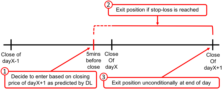

3.2 The next-day exit trading program

Based on Fig. 2, the corresponding trading program, in Multicharts’ Powerlanguage [16], is in Fig. 3. This next-day exit trading program has parameters SL and SS as the percentage of stop-loss for buy and short positions. When the difference between the current price and the predicted price exceeds numSD multiple of standard deviation, we initiate a new buy (or short) position. Length specifies the period to measure the standard deviation.

In the trading program, D2price is the predicted price from deep learning models and is input as the second data source (called “data2” in Multicharts). $S$ is the standard deviation, while ok2buynextbar and ok2sellshortnextbar are two Boolean variables tracking whether buy or short decision is triggered. Line 7 of Fig. 3 determines if it is five minutes before the close, Line 9 decides whether to buy or short based on how far D2Price deviates from current price, Line 16 restricts the number of trades to once a day, Line 24 executes the possible stop-loss, and finally Line 31 forces exit at the end of trading day.

Optimization in program trading is conducted to find the maximum profit as the profitability that a deep learning model (with specific parameters) can reach.

3.2.1 Data collection of the three traded merchandise

Based on Pant [1] and the data collected, three commonly traded commodities, gold, soybean, and crude oil, are used for the experiments in this paper with their exact trading specification provided in Table 3.

Table 3
Data specification of three merchandises

Trading days	Soybean	Crude oil	Gold
	Monday – Friday	Monday – Friday	Monday – Friday
Trading hours	19:00 of prior day $\sim$ 13:20	17:00 of prior day $\sim$ 16:00	18:00 of prior day $\sim$ 17:00
Big point value	50 USD	1000 USD	100 USD
Data source	GLOBEX soybean Futures	GLOBEX crude-oil Futures	GLOBEX gold Futures
	provided by e-signal	provided by e-signal	provided by e-signal
Period	2006/01/01 $\sim$ 2018/04/30	2007/03/01 $\sim$ 2018/04/30	2007/03/01 $\sim$ 2018/04/30

Figure 3.

The code for the next-day exit trading program.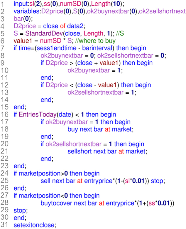

Both the daily close price and the price of five minutes before daily close are input for our deep learning models. All the collected price data is one-minute data since the program in Fig. 3 should be executed on one-minute data for correctness as required by Multicharts [16]. We use eighty percent of data for training and twenty percent for testing.

3.3 Parameter settings for LSTM and TCN models

In this work, the CudnnLSTM in Cudnn library of GPU [18] is used as the LSTM model, where the ranges of parameter settings are in Table 4. Those for the TCN model are in Table 5.

Table 4
Parameter setting for LSTM

Hidden layer	1					2
# of neuron	3	6	7	50	80	3	6	7	50	80

Table 5

Parameter setting for TCN

Activation functions	ReLu, SeLu
Filters	32, 64, 128, 256, 512, 1024
Dilations	[1, 2, 4, 8], [1, 2, 4, 8, 16], [1, 2, 4, 8, 16, 32], [1, 2, 4, 8, 16, 32, 64], [1, 2, 4, 8, 16, 32, 64, 128],
	[1, 2, 4, 8, 16, 32, 64, 128, 256], [1, 2, 4, 8, 16, 32, 64, 128, 256, 512]
Dropout_rate	0, 0.2, 0.5, 0.7

3.4 Measuring errors for the prediction models

Based on the typical quality measures as discussed in Section 2.6 and the available open-source codes for further modification, we use the coefficient of determination ( $R^{2}$ ) from scikit-learn library where $R^{2}=r2\_\textit{score}\left({y_{\textit{test}},y_{\textit{test\_pred}}}\right)$ , and the code of $\textit{MASE}\left({\textit{train},\textit{test},\textit{pred}}\right)$ from Davidson-Pilon [19]. Its calculation includes the following steps: (1) calculate the length $n$ of train data set, (2) use the diff function from numpy to mimic naïve prediction (calculate continuous residuals), (3) sum up the mimicked naïve forecast, take absolute value, and divide by n-1 to get the denominator of MASE, and (4) similarly calculate the residuals among test and test_pred, take absolute value, use mean to sum and average, and finally divide by the denominator as acquired in (3) to get MASE.

4. Experiments and discussion

Using the parameter sets for LSTM in Section 3.3 and the error measurement of $R^{2}$ and MASE, the results of three merchandises in Table 3 are presented in Table 6 and Fig. 4. We use eighty percent of data as training sets, and twenty percent as test sets. All three merchandises show high $R^{2}$ in the training set with $R^{2}$ dropped for certain parameter settings in their test sets. MASE and $R^{2}$ reveals similar trends

When reading Fig. 4 for the results from test sets, the more points at the right lower corner the better for the merchandise since the more close to 1 the better for $R^{2}$ , and the more close to 0, the better for MASE. Thus, models for both gold and soybean reveal an excellent learning effect in LSTM, but not the case for crude oil.

Table 6
Comparing results of LSTM

Hidden layer	1	1	1	1	1	2	2	2	2	2
neuron	3	6	7	50	80	3	6	7	50	80
Gold
Train	0.994	0.994	0.994	0.994	0.991	0.993	0.993	0.992	0.989	0.988
Test	0.965	0.967	0.966	0.968	0.945	0.963	0.965	0.965	0.94	0.94
MASE	0.764	0.746	0.759	0.733	1.028	0.802	0.775	0.758	1.087	1.085
Soybean
Train	0.975	0.981	0.977	0.977	0.981	0.97	0.978	0.978	0.981	0.982
Test	0.911	0.921	0.946	0.947	0.946	0.784	0.886	0.87	0.945	0.951
MASE	0.68	0.647	0.497	0.492	0.491	1.196	0.822	0.887	0.499	0.462
Crude oil
Train	0.992	0.992	0.993	0.993	0.993	0.99	0.992	0.993	0.992	0.991
Test	0.903	0.955	0.974	0.97	0.976	0.858	0.907	0.956	0.978	0.98
MASE	1.614	1.224	0.921	0.954	0.873	1.963	1.573	1.102	0.874	0.849

Table 7

Comparing results for activation functions of TCN

Activation function	SeLu	ReLu
Gold
Train	0.988	0.985
Test	0.966	0.963
MASE	0.753	0.797
Soybean
Train	0.975	0.975
Test	0.94	0.909
MASE	0.526	0.652
Crude oil
Train	0.992	0.979
Test	0.974	0.484
MASE	0.95	4.132

Figure 4.

Error measurement for the test set from LSTM.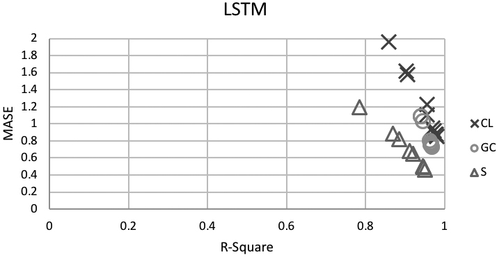

Parameter sets for the TCN models in Section 3.3 are also applied to the same three merchandises. TCN’s parameter setting includes activation function, filters, dilations, and dropout rate, which are evaluated individually.

Activation functions, SeLu and ReLu, are compared in Table 7. All three merchandise shows high $R^{2}$ in the training set. SeLu performs better than ReLu in the test sets for both soybean and crude oil, where both SeLu and ReLu perform similarly in gold. MASE also reveals the same trend. Here the setting for Filter is 256, 32 for Dilations, and 0.2 for the dropout rate. These values for Filters, Dilations, and dropout_rate are fixed as these values show better results when tested individually. When comparing the error measurement for different parameter settings, we use a similar approach. The purpose here is to know which parameter settings in TCN are of lower error measurement on the three merchandise.

Filters for TCN are compared as in Table 8. For test sets, gold has good results on all Filter parameters, crude oil performs well at around 128 to 512, and soybean performs well at most values except 1024. MASE also reveals the same trend. Here the setting of other parameters is SeLu, Dilations: 32, and Dropour_rate: 0.2.

Dilations for TCN are compared as in Table 9. For test sets, gold has good results on all Dilations parameters, crude oil performs well at 16, 32, and 256, and soybean performs well at 8, 16, and 32. MASE also reveals the same trend. Here the setting of other parameters is SeLu, Filters: 256, and Dropour_rate: 0.2.

Dropout_rate for TCN is compared as in Table 10. For test sets, gold has good results at 0.2 and 0.5, and crude oil and soybean both perform well at 0.2. MASE also reveals the same trend. Here the setting of other parameters is SeLu, Filters: 256, and Dilations: 32.

All the parameter sets mentioned above are applied to the trading program to calculate its profitability. We can then examine the relationship between traditional error measurement ( $R^{2}$ and MASE) and profitability.

Table 8

Comparing results for parameter sets of Filters of TCN

Filters	32	64	128	256	512	1024
Gold
Train	0.993	0.991	0.988	0.988	0.984	0.985
Test	0.969	0.969	0.968	0.966	0.962	0.956
MASE	0.704	0.705	0.731	0.753	0.806	0.887
Soybean
Train	0.953	0.968	0.973	0.975	0.975	0.969
Test	0.924	0.919	0.925	0.94	0.924	0.878
MASE	0.638	0.631	0.628	0.526	0.614	0.834
Crude oil
Train	0.988	0.988	0.991	0.992	0.992	0.987
Test	0.681	0.852	0.928	0.974	0.947	0.742
MASE	2.426	2.132	1.597	0.95	1.467	2.933

Table 9

Comparing results for parameter sets of Dilations of TCN

Dilations	8	16	32	64	128	256	512
Gold
Train	0.99	0.988	0.988	0.986	0.985	0.978	0.976
Test	0.968	0.966	0.966	0.966	0.963	0.957	0.953
MASE	0.724	0.749	0.753	0.744	0.796	0.87	0.925
Soybean
Train	0.976	0.974	0.975	0.966	0.96	0.954	0.94
Test	0.949	0.921	0.94	0.91	0.928	0.885	0.897
MASE	0.48	0.595	0.526	0.721	0.612	0.846	0.771
Crude oil
Train	0.992	0.992	0.992	0.992	0.992	0.992	0.989
Test	0.94	0.976	0.974	0.895	0.952	0.971	0.896
MASE	1.46	0.906	0.95	1.567	1.156	0.988	1.973

Table 10

Comparing results for parameter sets of Dropout_rate of TCN

Dropout_rate	0	0.2	0.5	0.7
Gold
Train	0.981	0.988	0.99	0.991
Test	0.958	0.966	0.967	0.946
MASE	0.857	0.753	0.729	0.933
Soybean
Train	0.945	0.975	0.929	0.641
Test	0.834	0.94	0.639	$-$ 0.224
MASE	1.04	0.526	1.562	3.124
Crude oil
Train	0.986	0.992	0.991	0.987
Test	0.796	0.974	0.893	0.773
MASE	3.065	0.95	1.492	3.247

Table 11

Performance summary of all models for three merchandises

	LSTM	TCN
Gold
Max. profit	15535	20990
Avg. profit	10749	15672
Standard dev.	5550	3835
Avg. MDD	12217	10540
Soybean
Max. profit	11925	13775
Avg. profit	8485	10255
Standard dev.	3578	2854
Avg. MDD	5561	6446
Crude oil
Max. profit	34897	20896
Avg. profit	15596	17195
Standard dev.	10568	6410
Avg. MDD	21435	12716

4.1 Relationships between the profitability of predicted prices and their error measurement

From the previous results, $R^{2}$ and MASE both demonstrate the same trend on almost all parameter sets. For simplicity, we only use $R^{2}$ as the error measurement when studying the relationship between profitability and traditional error measurement.

To evaluate the profitability of deep learning models, we use two years’ out-sample data with the trading program in Fig. 3 for initial capital of 100,000.0 US dollars to get the profitability of all the parameter sets of LSTM and TCN models in Tables 4 and 5. The average and maximum profitability for three merchandise in all models and parameter sets are in Table 11.

Figure 5.

Relationship of profitability and error measurement on gold.

Figure 6.

Relationship of profitability and error measurement on soybean.

Figure 7.

Relationship of profitability and error measurement on crude oil.

As Compared to LSTM, TCN provides higher profitability for gold. The standard deviation of the profitability and the averaged maximum drawdown (MDD) for TCN are both better than those from LSTM. The relationship between profitability and error measurement for models on gold is in Fig. 5. The (orange-colored) circles represent LSTM, and the (blue) triangles are for TCN. More dots at upper right corners indicate their models are with a higher positive correlation between profitability and error measurement (i.e., lower error leads to higher profits). For gold, this correlation coefficient is $-$ 0.55 for LSTM and 0.25 for TCN. When (hidden layers, # of neuron) $=$ (1, 80), (2, 50), (2, 80), the LSTM model gets highest profit. The highest one for TCN is (SeLu, 256, [1, 2, 4, 8, 16, 32], 0.2).

Soybean’s TCN models provide higher profitability than LSTM’s, and their standard deviation is also smaller. The relationship between profitability and error measurement for models of soybean is in Fig. 6. For soybean, the correlation coefficient is $-$ 0.24 for LSTM and 0.2 for TCN. When (hidden layers, # of neurons) $=$ (2, 80), the LSTM model gets the highest profit. The highest one for TCN is also (SeLu, 256, [1, 2, 4, 8, 16, 32], 0.2).

The profitability patterns of Crude oil from LSTM models are quite unstable. TCN models of crude oil provide higher averaged profitability. The standard deviation for the profitability and the averaged maximum drawdown (MDD) for TCN are both better than those from LSTM. The relationship between profitability and error measurement of corresponding models of crude oil is in Fig. 7. For crude oil, the correlation coefficient is $-$ 0.82 for LSTM and 0.01 for TCN. When (hidden layers, # of neuron) $=$ (2, 3) (2, 6), the LSTM model gets the highest profit. The highest one for TCN is also (SeLu, 256, [1, 2, 4, 8, 16, 32], 0.2).

From these analyses, we have the following findings: (1) TCN models provide a more positive correlation between profitability and error measurement ( $R^{2}$ ), (2) parameter sets from TCN provides much stable profitability than LSTM, especially the parameter set (SeLu, 256, [1, 2, 4, 8, 16, 32], 0.2) of TCN get the highest profitability in all three merchandise, (3) profitability fluctuates greatly in crude oil as well as its error measurement from both LSTM and TCN models. The correlation between profitability and error measurement for crude oil is also the most unstable among the three tested merchandise.

5. Conclusion

In this work, a new validation approach is proposed to evaluate the quality of deep learning models. The proposed method explores the relationships between the profitability and error measurements of deep learning models. “More precise prediction leads to better profitability” is a common hidden assumption for price prediction from deep learning where usually only the error between the predicted and actual prices is used to measure the quality of learning results. We re-evaluate this common assumption through our proposed validation approach. Validation approaches similar to ours can be used by others to add a new dimension of quality measurements for deep learning models. Our approach emphasizes that the application results of the predicted values from deep learning are also one of the critical quality measurements.

A three-stage process of validation, as proposed in Section 3, is conducted on three commonly traded merchandise in this paper, with all experiment results displayed and analyzed in Section 4. Program trading measures the profitability of learning models. We use a next-day exit trading program in this paper to match the deep learning prediction model.

From these analyses, we have the following findings: (1) TCN models provide a more positive correlation between error measurement ( $R^{2}$ ) and profitability. (2) Parameter sets from TCN provide much stable profitability than LSTM, especially the parameter set (SeLu, 256, [1, 2, 4, 8, 16, 32], 0.2) of TCN gets the highest profitability in all three merchandise. (3) Profitability fluctuates greatly in crude oil as well as its error measurement from both LSTM and TCN models. The correlation between profitability and error measurement for crude oil is also the most unstable among the three tested merchandise. (4) With given parameter sets, if merchandise (gold and soybean) is of low averaged magnitude error, then its profitability is more stable. If it is of a more significant magnitude error (crude oil), then its profitability is unstable. (5) TCN outperforms LSTM in almost all our cases. (6) A highly positive correlation does not exist between profitability and error measurement. Finally, (7) how the applications use predicted values and their application results better be part of the quality measurement for deep learning.

The focus of this work is to address the loose relationship between the error measurement of predicted values and the trading profitability. As for the absolute trading return of our proposed trading strategy, they are at around 7%–8% annual return based on Table 11, which is similar to those in [6]. The absolute return rate may further increase if domain experts are more involved during stages 2 and 3 for the proposed three-stage process. As it is not the focus of this work, we do not perform tasks that way.

A final note is that the quality of predicted prices from deep learning and how the predicted prices lead to profitability could be, in fact, two different issues. For example, we have conducted similar experiments on the 15 key Taiwan stocks with 30 years of data. Though the predicting quality (measured in MSE and $R^{2}$ ) are similar to this work; we achieve better trading profitability when (1) the predicting span is extended to one week, (2) the holding period is extended longer, and (3) the buying price is proportionally set lower than the predicted.

References

Pant

, A Guide For Time Series Prediction Using Recurrent Neural Networks (LSTMS), 2017, Retrieved on https://blog.statsbot.co/time-series-prediction-using-recurrent-neural-networks-lstms-807fa6ca7f.

Schoneburg

, Stock price prediction using neural networks: A project report, Neurocomputing 2 (1990), 17–27.

Leinweber

D.J.

, Stupid data miner tricks: Overfitting the S&P 500, The Journal of Investing Spring 2007 16 (2007), 15–22.

LeCun

Bengio

and Hinton

, Deep learning, Proceedings of Nature 521 (2015), 436–444.

Greff

Srivastava

R.K.

Koutnik

Steunebring

B.R.

and Schmidhuber

, LSTM: A search space odyssey, Proceedings of IEEE Transactions on Neural Networks and Learning Systems 28 (2017), 2222–2232.

Shen

and Zhu

, Stock Price Prediction Using Attention-based Multi-Input LSTM, in: Proceedings of The 10th Asian Conference on Machine Learning (PMLR 95), 2018, pp. 454–469.

Walter

Ritter

and Schulten

, Non-linear Prediction with Self-organizing Maps, in: IJCNN International Joint Conference on Neural Networks, 1990, pp. 17–21.

Chollet

, Perspective on DEEP LEARNING with Python, 2017.

Bai

Kolter

J.Z.

and Koltun

, An Empirical Evaluation of Generic Convolutional and Recurrent Networks for Sequence Modeling, arXiv: 1803.01271v2, 2018.

10.

Schmidhuber

, Deep learning in neural nerworks: An overview, Neural Networks 61 (2015), 85–117.

11.

Krizhevsky

Sutskever

and Hinton

G.E.

, ImageNet Classification with Deep Convolutional Neural Network, in: Proceedings of the 25th International Conference on Neural Information Processing Systems (NIPS’12), Vol. 1, 2012, pp. 1097–1105.

12.

Hochreiter

Klambauer

Unterthiner

and Mayr

, Self-normalizing neural networks, Proceedings of NIPS’17 Advances in Neural Information Processing Systems 30 (2017).

13.

Brownlee

, Perspective on Better Deep Learning, 2019.

14.

Hyndman

R.J.

and Koehler

A.B.

, Another look at measures of forecast accuracy, Proceedings of International Journal of Forecasting 22(4) (2006), 679–688.

15.

Keith

, Perspective on Trading program for interacting with market programs on a platform, 2000.

16.

Multicharts, 2019, retrieved on https://www.multicharts.com/.

17.

Pardo

, Perspective on The Evaluation and Optimization of Trading Strategies 2nd, 2008.

18.

NVIDIA, cuDNN Developer Guide, 2018, Retrieved on https://docs.nvidia.com/deeplearning/sdk/cudnn-developer-guide/index.html.

19.

Davidson-Pilon

, Computes the MEAN-ABSOLUTE SCALED ERROR forecast error for univariate time series prediction, 2013. Retrieved from https://github.com/CamDavidsonPilon/Python-Numerics/blob/master/TimeSeries/MASE.py.