Deep hierarchical spectral-spatial feature fusion for hyperspectral image classification based on convolutional neural network

Abstract

Joint spectral-spatial feature extraction has been proven to be the most effective part of hyperspectral image (HSI) classification. But, due to the mixing of informative and noisy bands in HSI, joint spectral-spatial feature extraction using convolutional neural network (CNN) may lead to information loss and high computational cost. More specifically, joint spectral-spatial feature extraction from excessive bands may cause loss of spectral information due to the involvement of convolution operation on non-informative spectral bands. Therefore, we propose a simple yet effective deep learning model, named deep hierarchical spectral-spatial feature fusion (DHSSFF), where spectral-spatial features are exploited separately to reduce the information loss and fuse the deep features to learn the semantic information. It makes use of abundant spectral bands and few informative bands of HSI for spectral and spatial feature extraction, respectively. The spectral and spatial features are extracted through 1D CNN and 3D CNN, respectively. To validate the effectiveness of our model, the experiments have been performed on five well-known HSI datasets. Experimental results demonstrate that the proposed method outperforms other state-of-the-art methods and achieved 99.17%, 98.84%, 98.70%, 99.18%, and 99.24% overall accuracy on Kennedy Space Center, Botswana, Indian Pines, University of Pavia, and Salinas datasets, respectively.

Keywords

CNN deep learning feature fusion feature extraction hyperspectral image classification informative bands

1. Introduction

Hyperspectral images (HSIs) consist of several hundreds of continuous spectral bands across the entire electromagnetic spectrum, which provide wealth of information and helps in distinguishing objects or physical materials [1]. It has several applications such as environment observing [2], military purpose [3], agriculture [4]. On the other hand, HSIs also present inherent challenges, such as information redundancy, uncertainty, high dimensionality, varying spatial dimensions, interclass similarity, intraclass diversity, variations within the same class spectrum, and limited availability of labeled samples. However, one of the major task in the application of HSI is classification, which targets to assign a particular class to every image pixel. To classify the pixel, various HSI classification methods have been proposed such as support vector machine (SVM) [5, 6], sparse representation classifier [7]. Meanwhile, extreme learning machine (ELM), active learning [8], and other methods have been introduced and shown satisfactory performance. But, due to the presence of same spectrum of different objects and different spectrum of same objects, it was difficult for the methods to distinguish objects efficiently as they were relied only on spectral information [9, 10]. For this reason, poor classification accuracy has been reported by many methods. However, with the advancement of imaging technology, HSI sensors can exploit spatial information, which is another useful information resource. Early attempts for extracting spatial feature in HSI classification have shown improved classification performance [11, 12, 13]. But, it has been observed that depending only on spatial information also makes it hard to identify all types of objects due to complex distribution of spatial structure. Therefore, several studies in the past have suggested to consider both spectral and spatial features for improving the representation capability of HSIs.

During the past decades, various studies were carried out based on spectral-spatial features. But, the early spectral-spatial based classification approaches were relied on shallow features, which were unable to represent semantic information. Recently, various deep learning methods, such as stacked autoencoder (SAE) [9], deep belief network (DBN) [14] and convolutional neural network (CNN) [15, 16, 17, 18, 19], have shown excellent performance in various applications. These deep learning methods have been extensively used as powerful feature extraction methods. Compared with traditional methods, deep learning methods [20, 21, 22, 23, 24, 25] are much efficient for extracting abstract and semantic features. Therefore, HSI classification using these deep learning methods have shown great research interest in recent times.

For instance, in [9], a SAE based deep learning framework was proposed to extract joint spatial-spectral features. Chen et al. [14] presented DBN based model by training multiple layer’s through restricted Boltzmann machine network. To extract spatial information, SAE and DBN follows the same neighboring structure by converting image cube into 1D vectors. Therefore, it has limitation on spatial feature extraction. On the contrary, CNN can efficiently extract the spatial information through local connections and reduce the number of parameters by using shared weights [15]. Thus, CNN has attracted particular research interest in HSI classification [26, 27, 28, 29, 30, 31]. In [26], a CNN is adopted for spectral-spatial feature extraction of a pixel after applying the Randomized PCA and classification is done through multi-layer perceptron. Li et al. [27] presented a fully CNN based framework which enhances deep features via convolutional, deconvolutional and pooling layers. In [28], a HSI reconstruction model has been built by using deep CNN for improving the spatial feature, which follows ELM for classifying the image. Yu et al. [29] integrated hash features in a CNN framework which utilizes semantic information to enhance the classification performance. In [30], Chen et al. introduced 1D CNN, 2D CNN and 3D CNN to effectively learn the deep spectral and spatial features in the perspective of HSI classification. In 3D CNN, simultaneous extracting of spectral and spatial features may cause the loss of spectral information [31]. Therefore, to address this problem, we need to extract spectral and spatial features separately.

After spectral-spatial feature extraction, feature fusion is another important step for HSI classification [32, 33, 34, 35, 36, 37, 38, 39, 40, 41, 42, 43]. In [32], a dual channel CNN method was proposed for extracting spectral and spatial features through 1D CNN, and 2D CNN, respectively and fused them together. Hao et al. [33] have proposed two channel framework with fusion scheme. The two channel framework includes stacked denoising autoencoder for encoding spectral information and CNN for spatial feature extraction. The extracted features from these two models were fused by adaptive-class specific weight. Xu et al. [34], presented a fusion scheme where the features from HSI and other sensor’s data (e.g. light detection and ranging) were extracted through CNN and cascade block CNN, respectively. Song et al. [35], proposed a fusion network where residual learning has been introduced to optimize the several convolutional layers and fused the output of different hierarchical layers to improve the classification accuracy. Cheng et al. [37] also improved the classification performance by adopting the off-the-shelf CNN models and unified metric learning based framework. In [38], the unsupervised cooperative sparse autoencoder was presented for fusing spatial context and raw spectral information. In [39], a novel fusion scheme was proposed. It utilized complimentary information of subpixel, pixel and superpixel for HSI classification. Li et al. [40] fused the spectral-spatial and texture features to complete the HSI classification. Recently, Zou et al. [41] adopted a fusion technique by utilizing fully 3D convolutional neural network to extract spectra-spatial and semantic information for HSI classification. From these fusion strategies, it can be concluded that fusion can be a effective choice to enhance the classification performance of HSI.

Nevertheless, optimal number of bands is an important criterion for visual recognition, especially when HSI is considered. The HSI classification models proposed in literature [30, 44] employed excessive number of bands for feature extraction, but these models were not fully able to extract the discriminative features due to mixing of informative and less informative (or noisy) bands. Further, the use of excessive bands may cause negative effects such as overfitting, performance degradation, and high computational cost.

To overcome the aforementioned drawbacks, we proposed a novel deep hierarchical spectral-spatial feature fusion (DHSSFF) method to classify HSIs. In DHSSFF, specific features were extracted separately through two different CNN based architectures, where 1D CNN is used to extract spectral features by considering entire spectral bands and 3D CNN is employed for extracting spatial features from few informative bands. Then, the extracted deep features from two architectures were fused to retain the discriminative feature followed by predicting the class level. This paper’s major contributions are summarized as follows.

Proposed a model named DHSSFF, where deep spectral and spatial features are extracted through 1D CNN and 3D CNN, respectively, to generate the accurate classification result.

To make full use of spectral and spatial information, proposed model focuses on deep feature fusion which can merge the detailed information of shallow layers and semantic information of deep layers.

Investigation of effect of number of bands on the performance of proposed model.

Investigation of effect of number of training samples on the performance of proposed model.

Extensive comparison of our model with the literature on five widely used HSI datasets.

The remaining part of this paper is organized as follows. Section 2 outlines our proposed method, which contains entire spectral band based 1D CNN, few informative band based 3D CNN, and fusion of deep spectral-spatial features for HSI classification. Section 3 demonstrates the experimental results and analysis followed by conclusion in Section 4.

2. Proposed methodology

In this section, we have presented a novel DHSSFF model for HSI classification. Here, the deep spectral features were extracted via 1D CNN by considering entire spectrum signatures. On the other hand, few informative bands were selected using principal component analysis (PCA) [45] to extract deep spatial features through 3D CNN. The reason for selection of PCA over other algorithms for hyperspectral image is its ability to effectively reduce dimensionality while preserving significant spectral information, its simplicity, interpretability and its widespread acceptance. At last, we have adopted a fusion technique to take full advantage of deep spectral-spatial features. In the following sections, a brief description has been provided of CNN model. Then, the details of entire spectral band based 1D CNN (ESB1DCNN) has been provided followed by few informative band based 3D CNN (FIB3DCNN). Finally, the proposed DHSSFF model has been presented.

2.1 CNN

In general, the CNN is constructed by alternate stacking of convolutional layers, pooling layers followed by fully connected (FC) layers. Let $X$ be the input image of $M \times N \times B$ size, where $M \times N$ refers to spatial dimension of the image, and B denotes the number of bands. Now, suppose there are $k$ filters in a particular convolutional layer represented as $W$ and the bias term is represented as $b$ , then $m$ th feature map ( $x_{m}$ ) can be expressed by Eq. (1).

\begin{aligned} x_{m} = \sum_{n = 1}^{B} α (x_{n} * w_{m} + b_{m}), m = 1, 2, \dots k . \end{aligned}

(1)

where,

x_{n}

is the

n

th feature map,

w_{m}

and

b_{m}

are the

m

th element of

W

and

b

, respectively,

*

operator denotes the convolutional operation, and the activation function is represented by

α

. The most popular activation function Rectified linear unit (ReLU) is utilized to enhance the nonlinearity, which is defined as:

\begin{aligned} α (x) = max (0, x) \end{aligned}

(2)

After utilizing activation function, the pooling operation progressively downsizes the spatial dimension of the feature maps, which deals with minimizing the computation cost. The most common pooling method in HSI classification is max pooling [46] which picks strongest value from the pooling region to hold the discriminative features. Generally, after several convolutional and pooling operations, FC layers are considered at the top of the network. FC layer combines all the feature maps generated from its previous layer by converting them into a feature vector. Finally, the feature vector is transferred to the softmax layer to produce the probability distribution of each class.

2.2 Entire spectral band based 1D CNN (ESB1DCNN)

In this paper, we have introduced a ESB1DCNN model as shown in Fig. 1 for spectral feature extraction. Here, normalized image in the range [ $-$ 0.5, $+$ 0.5] has been taken as input by considering all the bands. This model has been constructed of alternate stacking of convolutional, and pooling layers followed by FC. The number of convolutional and pooling layers varies with the datasets on the basis of empirical study which has been discussed in Subsection 3.2. In each convolutional layer, 1D kernel has been used to effectively capture abstract spectral information towards the spectral dimensions. The output of the convolutional layer is feature maps, where a neuron’s value $n_{i j}^{a}$ at position a in the jth feature map of ith layer can be represented as follows:

\begin{aligned} n_{i j}^{a} = α (\sum_{k} \sum_{r = 0}^{R_{i} - 1} n_{(i - 1) k}^{a + r} * w_{i j k}^{r} + b_{i j}) \end{aligned}

(3)

where

k

is the feature map of

(i - 1)

th layer, which is connected with the ongoing feature map,

w_{i j k}^{r}

denotes the weight at position

r

linked with the

k

th feature map,

R_{i}

represents the width of the kernel, and

b_{i j}

is the bias term of

j

th feature map in

i

th layer.

Fig. 1.

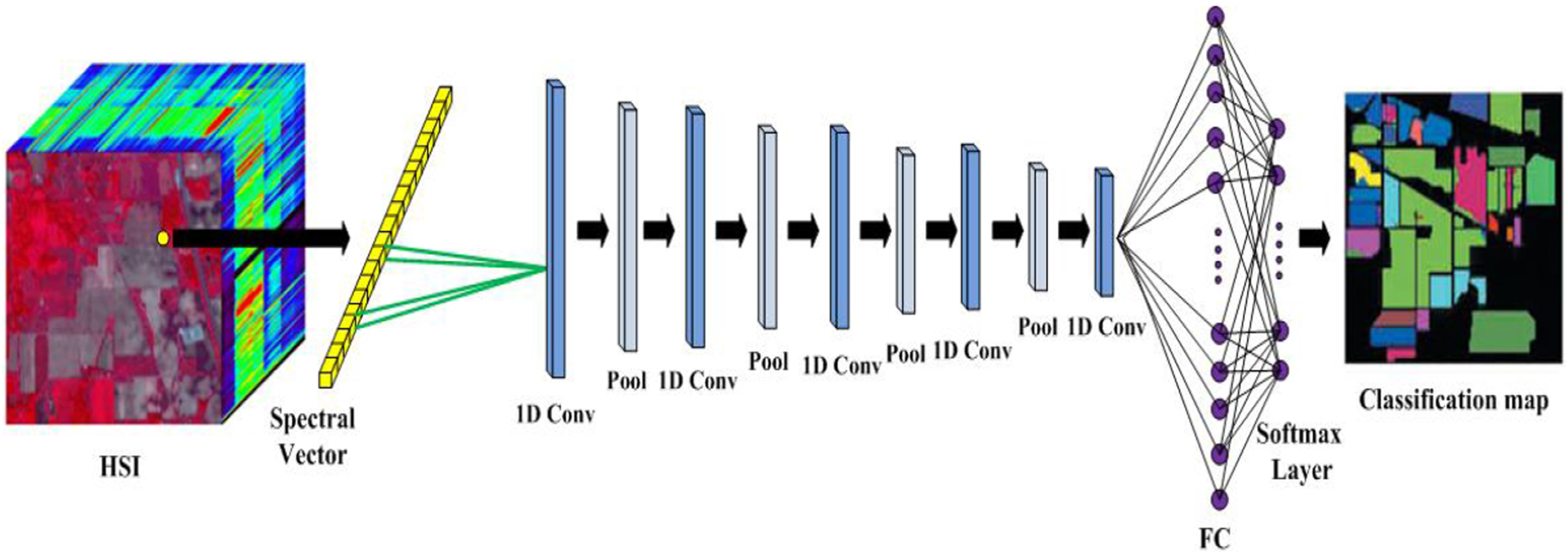
Architecture of ESB1DCNN model for spectral feture extraction.

Fig. 2.

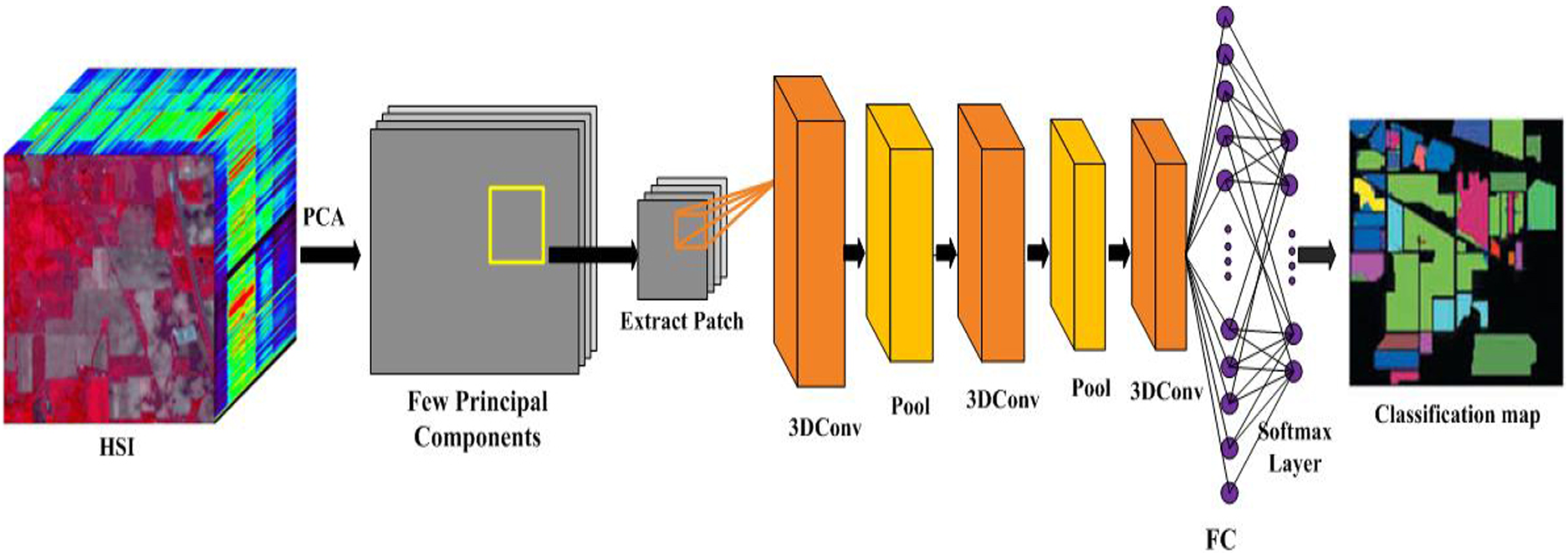
Architecture of FIB3DCNN model for spatial feture extraction.

2.3 Few informative band based 3D CNN (FIB3DCNN)

To extract spatial features, another model FIB3DCNN has been developed in this paper. The Fig. 2 shows the FIB3DCNN architecture. As a preprocessing step of HSI classification, we have performed normalization in the range of [ $-$ 0.5, $+$ 0.5] on the input image. Then, PCA has been applied to select the most informative bands which reduces the computational cost. After selecting informative bands, image patches of size (27 $\times$ 27) centered at the corresponding spectral pixels were cropped and has been considered as training samples. Then, 3D CNN has been employed for spatial feature extraction from the selected informative bands. In 3D CNN, the neuron’s value $n_{i j}^{a b c}$ at position $(a, b, c)$ of the $j$ th feature map in $i$ th layer is given by Eq. (4).

\begin{aligned} n_{i j}^{abc} = α (\sum_{k} \sum_{r = 0}^{R_{i} - 1} \sum_{s = 0}^{S_{i} - 1} \sum_{t = 0}^{T_{i} - 1} n_{(i - 1) k}^{(a + r) (b + s) (c + t)} * w_{i j k}^{rst} + b_{i j}) \end{aligned}

(4)

where

k

is the feature map of

(i - 1)

th layer, which is connected with the ongoing

j

th feature map, and

R_{i}

and

S_{i}

are the height and width of the convolutional kernel.

T_{i}

refers size of the kernel with respect to spectral dimension,

w_{i j k}^{r s t}

is the kernel value at position

(r, s, t)

, and

b_{i j}

is the bias term of the

j

th feature map in

i

th layer.

Considering the complex structure of HSI, our FIB3DCNN model consists of four convolutional layers, two pooling layers, and one FC layer to process the image patches. But, after processing of several convolutional and pooling operations, sudden conversion of convolutional (or pooling) layer to FC may lead to spatial information loss. Due to this, we have adopted multiple convolutional layers before FC layer, where both spatial and semantics information were exploited properly.

2.4 DHSSFF

In HSIs, the spectral bands of pixels of same class may vary due to the different imaging conditions, e.g., change in weather, environment, and temperature. Therefore, depending only on too few bands is critical for spectral-spatial feature extraction. On the contrary, spectral-spatial feature extraction requires several bands to be considered. However, excessive band may be associated with mixing of informative and non informative bands, which cannot provide desirable spectral and spatial features. For instance, when convolution operation is performed on HSI, any non informative band may lead to spectral information loss. Due to this, we have extracted spectral and spatial features separately using ESB1DCNN and FIB3DCNN, respectively and this dual channel model collectively called as DHSSFF model.

Fig. 3.

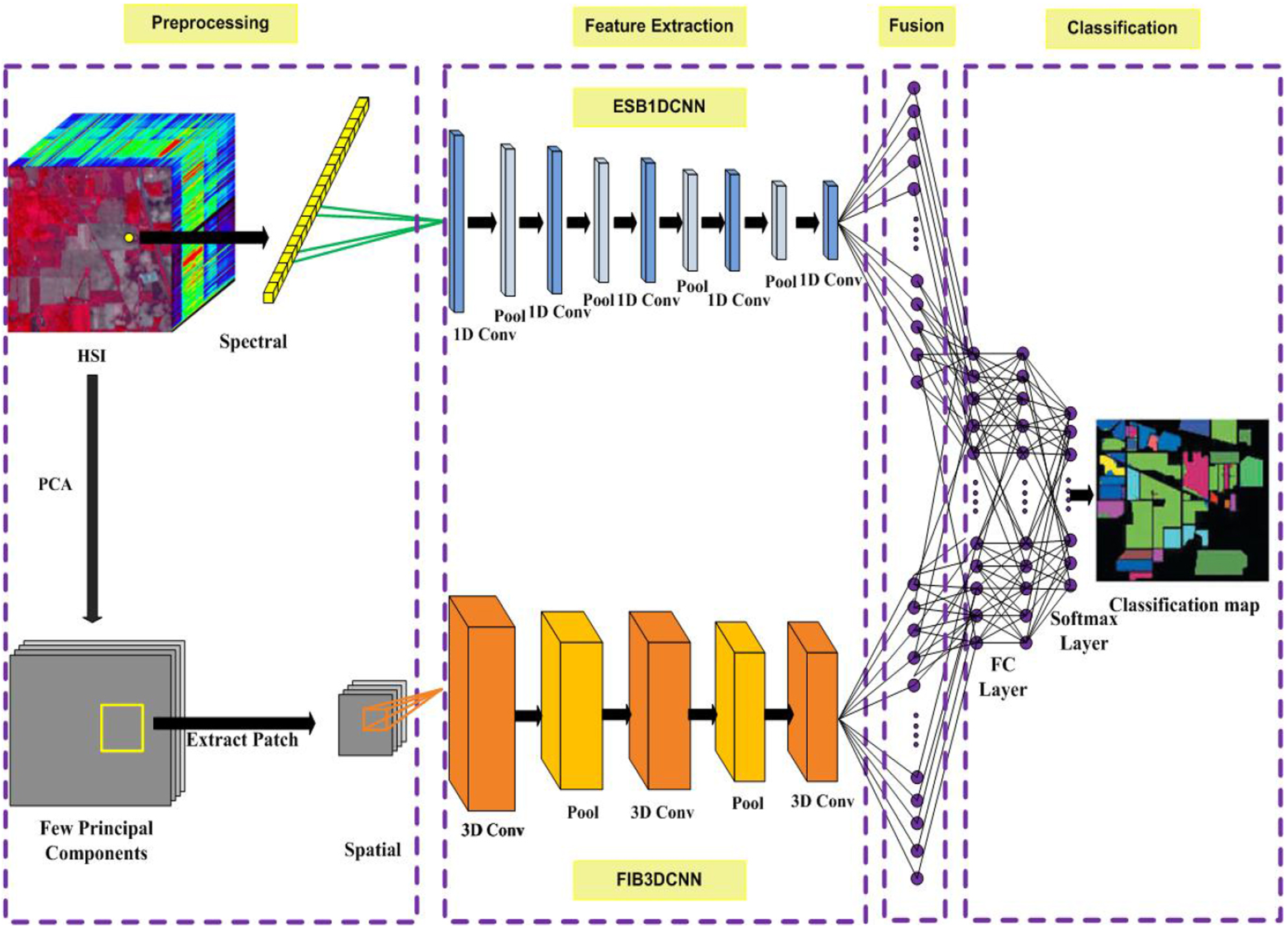
Architecture of the proposed DHSSFF model.

The architecture of DHSSFF model is shown in Fig. 3. The entire architecture is divided into four stages. In the first stage, preprocessing has been performed such as normalization and selection of informative bands using PCA for spatial feature extraction followed by patch extraction. The second stage is dedicated for feature extraction. The spectral features were extracted using ESB1DCNN and spatial features were extracted using FIB3DCNN. After that, a fusion scheme has been adopted to concatenate the deep features obtained from aforementioned two models which form a FC layer. In addition, we have considered two more FC layers for better representation of semantic information and lastly, a softmax classifier to predict the class label.

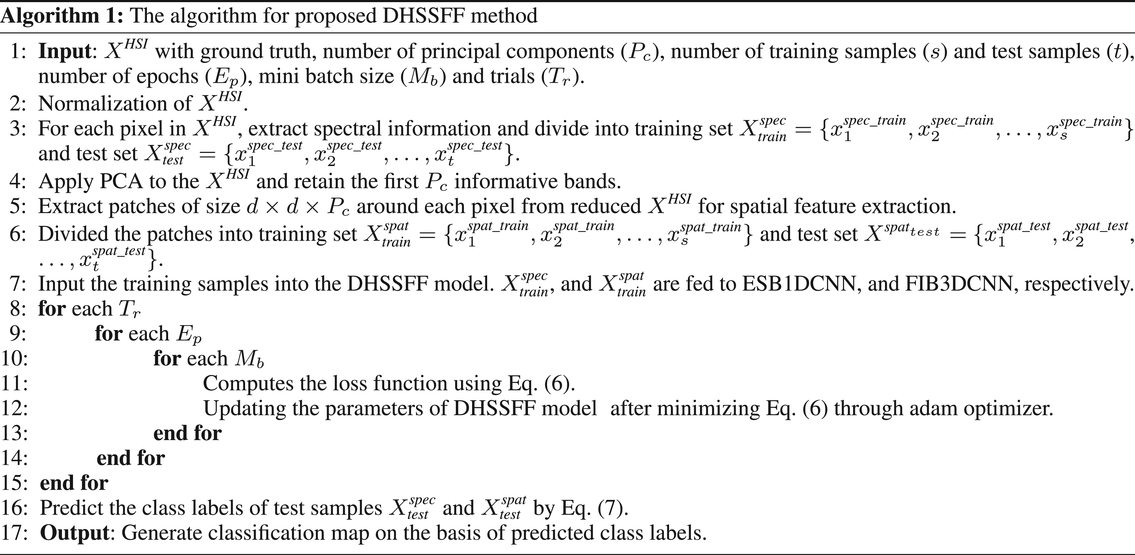
The pseudo code of DHSSFF model is represented in Algorithm 3. Let $X^{H S I} \in R^{M \times N \times B}$ be the HSI, where number of rows, columns and bands are denoted by $M$ , $N$ and $B$ , respectively. The input for the ESB1DCNN is spectral information of each pixel considering all the bands that can be denoted as $X^{S p e c} \in R^{1 \times 1 \times B}$ . In case of FIB3DCNN which extracts spatial features, PCA was applied to diminish the dimensionality of the image and first $P_{c} ≪ B$ informative bands were selected. The image with selected bands can be represented as $X^{S p a t} \in R^{M \times N \times P_{c}}$ . Further, a neighboring region with size of $d \times d \times P_{c}$ was considered for each pixel centered at $X^{S p e c}$ to extract image patches and fed to FIB3DCNN as input. Now, $X^{S p e c}$ and $X^{S p a t}$ has been partitioned into training and test set. Let us consider, $S$ be the total samples of a dataset and $s ≪ S$ number of samples to be selected for training, then training set for ESB1DCNN and FIB3DCNN can be represented by $X^{Spec_train} \in R^{s \times 1 \times 1 \times B}$ and $X^{Spat_train} \in R^{s \times d \times d \times P_{c}}$ , respectively i.e. the collective training samples can be represented as $x^{s} = {X^{Spec_train}$ , $X^{Spat_train}}$ and the class labels of $x^{s}$ can be encoded as $y^{s} \in Y$ where, $Y = {1, 2, \dots, C_{n}}, C_{n}$ is the number of classes. Let $F 1 \in R^{d 1}$ and $F 2 \in R^{d 2}$ be the feature vectors obtained from ESB1DCNN and FIB3DCNN, respectively, where d1 and d2 represents the dimensions. After fusion, the resultant feature vector can be represented by $F^{f u s e d} = {f_{i}^{1}, f_{i}^{2}, \dots, f_{i}^{d 1}, f_{i}^{1}, f_{i}^{2}, \dots, f_{i}^{d 2}} (i \in 1, 2)$ where $f_{i}^{k}$ is the $k$ th feature of the $i$ th channel. A softmax layer generates the probability distribution of each class as shown in Eq. (5).

\begin{aligned} q_{i}^{s} = \frac{e^{z_{i}^{s}}}{\sum_{j = 1}^{C_{n}} e^{z_{j}^{s}}}, i = 1, 2, \dots C_{n} . \end{aligned}

(5)

where

z_{i}^{s}

is the

i

th value of last FC layer. Then, the loss function is calculated by considering the cross entropy between true class probability (

y^{s}

) and predicted class probability (

q^{s}

), which is defined in Eq. (6). To minimize the loss function, adam optimizer has been utilized. After certain number of epochs, the training process is completed and the model is ready to predict the class labels of test samples

x^{t e s t} \in X^{H S I}

based on highest probability

q_{i}

with the help of Eq. (7).

\begin{matrix} L = - \frac{1}{s} \sum_{i = 1}^{s} [y_{i} \log (q_{i}) + (1 - y_{i}) \log (1 - q_{i})] \end{matrix}

(6)

\begin{matrix} C l a s s (x^{t e s t}) = a r g m a x q_{i}, i = 1, 2, \dots, C_{n} . \end{matrix}

(7)

3. Experimental results and analysis

3.1 Datasets

To show the effectiveness of our model, we have performed several experiments on five well known HSI datasets: Kennedy Space Center (KSC), Botswana (BOT), Indian Pines (IP), University of Pavia (UP) and Salinas (SA). The details of datasets are given below.

The KSC hyperspectral image was gathered by the Airborne Visible Infrared Imaging Spectrometer (AVIRIS) sensor over KSC, Florida, on March 23, 1996. This data set includes 176 bands after removing water absorption and noisy bands, which ranging from 0.4 to 2.5 $μ$ m. The spatial size of each band is 512 $\times$ 614 with spatial resolution of 18 m/pixel. Thirteen classes are considered for this scene. Figure 6(a) shows false color image of KSC dataset.

The BOT dataset was captured by the NASA EO-1 satellite over the Okavango Delta, Botswana. It contains 242 spectral bands with 0.4 to 2.5 $μ$ m wavelength range and has spatial size of 1476 $\times$ 256 pixels with spatial resolution of 30 m/pixel. Before analyzing, 97 water absorption and noisy bands were removed. As a result, a new dimension has been formed with 145 bands. The dataset has 14 land cover classes. Figure 7(a) shows false color image of BOT dataset.

The IP hyperspectral image was acquired by the AVIRIS sensor in June 1992 over the Indian Pines test site in North-western Indiana. This image is comprising of 220 spectral reflectance bands in the wavelength range from 0.4 to 2.5 $μ$ m and has a spatial size of 145 $\times$ 145 pixels with spatial resolution of 20 m/pixel. Before experimenting, total 20 bands were removed due to the water absorption and noise. This scene has included 16 land cover classes. Figure 8(a) shows false color image of IP dataset.

The UP image covers an urban area of the University of Pavia, Northern Italy. It was captured by the Reflective Optics System Imaging Spectrometer (ROSIS) sensor on July 8, 2002. This dataset has 115 spectral bands across the spectral range from 0.43 to 0.86 $μ$ m where 12 noisy bands were removed. The spatial dimension of this scene is 610 $\times$ 340 with spatial resolution of 1.3m/pixel. Figure 9(a) shows the false color image of UP dataset.

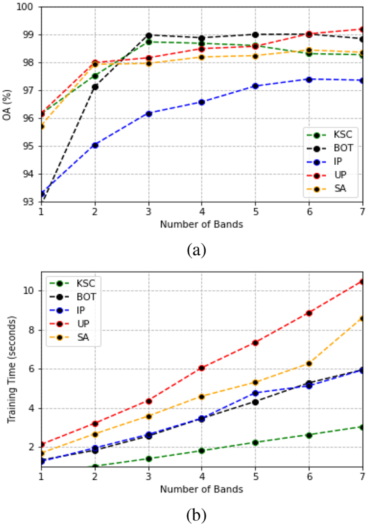
The SA dataset was also recorded by the AVIRIS sensor over the area of Salinas Valley, California, USA with a spectral range from 0.36 to 2.5 $μ$ m. It contains 224 spectral bands and has a size of 512 $\times$ 217 with spatial resolution of 3.7 m/pixel. For classification purposes, 16 classes were defined for this image. Before the experiments, 20 bands were removed due to the water absorption and noise. Figure 10(a) shows the false color image of SA dataset.

Fig. 4.

Sensitivity to the number of bands on FIB3DCNN for KSC, BOT, IP, UP, and SA datasets. (a) OA Vs number of bands. (b) Training time Vs number of bands.

3.2 Experimental design

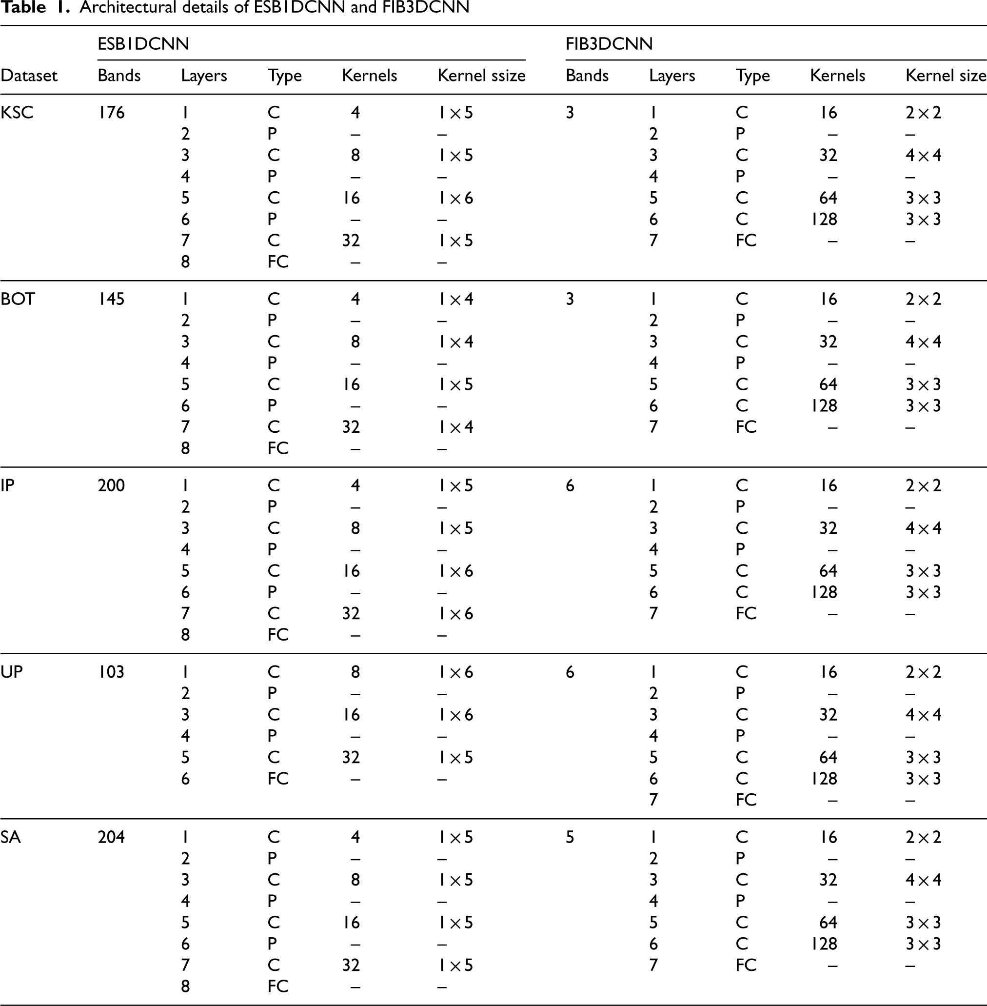
In our experiments, we empirically selected the parameters of ESB1DCNN, and FIB3DCNN. Table 1 shows the details of the architecture adopted for each dataset. In Table 1, the convolutional, pooling, and fully connected layers have been represented with C, P, and FC, respectively. For convolutional layer, the kernel size is varied according to the datasets. The max pooling of size 1 $\times$ 2 and 2 $\times$ 2 has been considered for all the pooling layers of ESB1DCNN and FIB3DCNN, respectively. In addition, following training parameters were set for all the experiments. The learning rate was set as 0.01 with weight decay of 1e-6. The experiments were performed for 200 epochs with mini batch size of 100. Further, we have repeated this process for 20 trials because partitioning of training and test samples were random and shown the standard deviation of performance parameters of 20 trials. In order to update the model parameters, the adam optimizer has been adopted.

Table 1
Architectural details of ESB1DCNN and FIB3DCNN

ESB1DCNN FIB3DCNN

Dataset Bands Layers Type Kernels Kernel ssize Bands Layers Type Kernels Kernel size

KSC 176 1 C 4 1 × 5 3 1 C 16 2 × 2

2 P – – 2 P – –

3 C 8 1 × 5 3 C 32 4 × 4

4 P – – 4 P – –

5 C 16 1 × 6 5 C 64 3 × 3

6 P – – 6 C 128 3 × 3

7 C 32 1 × 5 7 FC – –

8 FC – –

BOT 145 1 C 4 1 × 4 3 1 C 16 2 × 2

2 P – – 2 P – –

3 C 8 1 × 4 3 C 32 4 × 4

4 P – – 4 P – –

5 C 16 1 × 5 5 C 64 3 × 3

6 P – – 6 C 128 3 × 3

7 C 32 1 × 4 7 FC – –

8 FC – –

IP 200 1 C 4 1 × 5 6 1 C 16 2 × 2

2 P – – 2 P – –

3 C 8 1 × 5 3 C 32 4 × 4

4 P – – 4 P – –

5 C 16 1 × 6 5 C 64 3 × 3

6 P – – 6 C 128 3 × 3

7 C 32 1 × 6 7 FC – –

8 FC – –

UP 103 1 C 8 1 × 6 6 1 C 16 2 × 2

2 P – – 2 P – –

3 C 16 1 × 6 3 C 32 4 × 4

4 P – – 4 P – –

5 C 32 1 × 5 5 C 64 3 × 3

6 FC – – 6 C 128 3 × 3

7 FC – –

SA 204 1 C 4 1 × 5 5 1 C 16 2 × 2

2 P – – 2 P – –

3 C 8 1 × 5 3 C 32 4 × 4

4 P – – 4 P – –

5 C 16 1 × 5 5 C 64 3 × 3

6 P – – 6 C 128 3 × 3

7 C 32 1 × 5 7 FC – –

8 FC – –

	ESB1DCNN	FIB3DCNN
KSC	176	1	C	4	1 × 5	3	1	C	16	2 × 2
		2	P	–	–		2	P	–	–
		3	C	8	1 × 5		3	C	32	4 × 4
		4	P	–	–		4	P	–	–
		5	C	16	1 × 6		5	C	64	3 × 3
		6	P	–	–		6	C	128	3 × 3
		7	C	32	1 × 5		7	FC	–	–
		8	FC	–	–
BOT	145	1	C	4	1 × 4	3	1	C	16	2 × 2
		2	P	–	–		2	P	–	–
		3	C	8	1 × 4		3	C	32	4 × 4
		4	P	–	–		4	P	–	–
		5	C	16	1 × 5		5	C	64	3 × 3
		6	P	–	–		6	C	128	3 × 3
		7	C	32	1 × 4		7	FC	–	–
		8	FC	–	–
IP	200	1	C	4	1 × 5	6	1	C	16	2 × 2
		2	P	–	–		2	P	–	–
		3	C	8	1 × 5		3	C	32	4 × 4
		4	P	–	–		4	P	–	–
		5	C	16	1 × 6		5	C	64	3 × 3
		6	P	–	–		6	C	128	3 × 3
		7	C	32	1 × 6		7	FC	–	–
		8	FC	–	–
UP	103	1	C	8	1 × 6	6	1	C	16	2 × 2
		2	P	–	–		2	P	–	–
		3	C	16	1 × 6		3	C	32	4 × 4
		4	P	–	–		4	P	–	–
		5	C	32	1 × 5		5	C	64	3 × 3
		6	FC	–	–		6	C	128	3 × 3
							7	FC	–	–
SA	204	1	C	4	1 × 5	5	1	C	16	2 × 2
		2	P	–	–		2	P	–	–
		3	C	8	1 × 5		3	C	32	4 × 4
		4	P	–	–		4	P	–	–
		5	C	16	1 × 5		5	C	64	3 × 3
		6	P	–	–		6	C	128	3 × 3
		7	C	32	1 × 5		7	FC	–	–
		8	FC	–	–

To measure the performance of classification methods, we have adopted three popular indexes: overall accuracy (OA), average accuracy (AA), and kappa coefficient ( $K_{P}$ ). Specifically, the OA is calculated as the proportion of total number of accurately classified test samples and the entire test samples. The average of accuracies of each class is represented by AA. For $K_{P}$ , statistical calculation is introduced to measure the similarity among classification map and ground truth map. The experiments were performed using laptop with Intel^® Core(TM) i5-6200U 2.4-GHz CPU with 8 GB memory and an NVIDIA GeForce 940M. All the experiments were implemented using Keras 2.2.4 and Tensorflow 1.12.0 (backend library).

In order to verify the effectiveness of the proposed model DHSSFF, we have compared it with four methods, SVM with radial basis function (RBF-SVM), ESB1DCNN, FIB3DCNN, and spectral spatial 3D CNN (SS3DCNN) [30]. For RBF-SVM and ESB1DCNN, spectral information alone is used in HSI classification whereas spatial features were extracted using image patches (27 $\times$ 27) [30] from few informative bands in case of FIB3DCNN. In SS3DCNN, spectral and spatial features were exploited with same number of bands as used in FIB3DCNN model for fair comparison.

3.3 Sensitivity to the number of bands in FIB3DCNN

Considering too few band for classification may lead to unsatisfactory performance due to the information loss. On the other hand, use of excessive number of bands results in reduction of classification accuracy due to non-informative bands with increase in computational time. Hence, an empirical investigation of trade-offs between classification accuracy and computational time has been done to get the number of optimum bands for each dataset in FIB3DCNN. We have selected the most informative bands using PCA by applying different number of principal components from 1 to 7 as shown in Fig. 4(a) and recorded the OA and training time. After analyzing, we have observed that the classification accuracy gets decreasing after third band with increase in computational time for KSC dataset as depicted in Fig. 4(b). Therefore, we have set the number of bands for KSC dataset as 3. Similarly, the classification accuracy gets saturated or start decreasing after 3rd, 6th, 6th, and 5th bands for BOT, IP, UP, and SA dataset, respectively. Hence, the number of bands has been set as 3, 6, 6 and 5 for BOT, IP, UP, and SA dataset, respectively.

3.4 Sensitivity to the number of training samples

To get the better performance, a deep learning model needs huge number of labeled training samples. On the contrary, remote sensing image has very less number of labeled training samples. Therefore, the objective in HSI classification is to achieve high classification accuracy with as less training samples as possible. In order to select the training samples, we have presented here an analysis with varying proportions of training and test samples for five methods on five datasets.

Figure 5(a)–(e) shows overall accuracy obtained using five methods with varying proportions of training samples. For KSC, BOT, and IP datasets, 4%, 6%, 8%, 10%, and 12% samples as training sets were haphazardly chosen from each class. As UP and SA datasets consist of huge number of samples compared with KSC, BOT, and IP datasets, less training samples were selected for these datasets. The proportions of training samples considered as 1%, 2%, 3%, 4%, 5% for UP dataset and 1%, 1.5%, 2%, 2.5%, 3% for SA dataset. We have observed from Fig. 5(a)–(e) that the classification performance gets improved when number of training sample is increased for all the methods and for all the datasets. In addition, our observation in DHFFSS method is that the OA reaches above 99%, 98%, and 98% for KSC, BOT, and IP dataset, respectively when 10% training samples were selected. There is marginal improvement in OA when more than 10% training samples were considered with increased computational time. Therefore, we have found 10% training samples to be an optimal choice for KSC, BOT, and IP datasets. With similar observations, 4% and 2.5% training samples have been found the optimal proportion for UP and SA datasets, respectively. Moreover, similar behavior can be observed in case of other methods on all five datasets. Hence, all the experiments performed in this paper are based on these selected proportions of training samples.

Fig. 5.

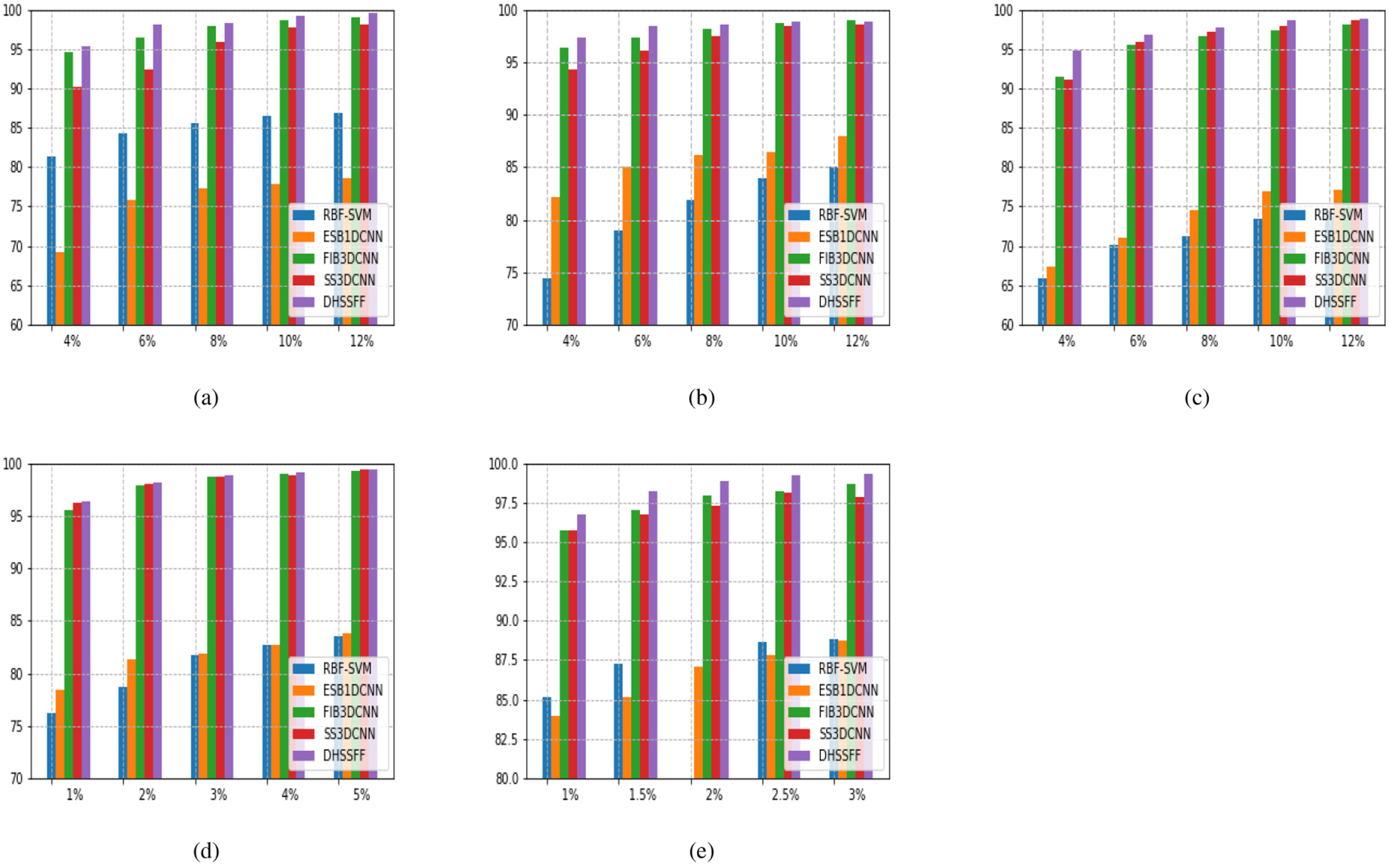
Sensitivity to the number of training samples using RBF-SVM, ESB1DCNN, FIB3DCNN, SS3DCNN, and DHSSFF methods. (a) KSC. (b) BOT. (c) IP. (d) UP. (e) SA.

3.5 Experimental results

3.5.1 Results on KSC dataset

The first experiment was performed on KSC dataset. All labeled samples were partitioned into training and test set. About 10% samples from each class were haphazardly selected to train the model, and rest samples were used as test set which is shown in Table 2.

Table 2
Number of training and test samples used in the KSC dataset

No. Class Training samples Test samples

1 Scrub 76 685

2 Willow swamp 24 219

3 CP hammock 26 230

4 CP/Oak 25 227

5 Slash pine 16 145

6 Oak/Broadleaf 23 206

7 Hardwood swamp 11 94

8 Graminoid marsh 43 388

9 Spartina marsh 52 468

10 Catiail marsh 40 364

11 Salt marsh 42 377

12 Mud flats 50 453

13 Water 93 834

Total 521 4690

No.	Class	Training samples	Test samples
1	Scrub	76	685
2	Willow swamp	24	219
3	CP hammock	26	230
4	CP/Oak	25	227
5	Slash pine	16	145
6	Oak/Broadleaf	23	206
7	Hardwood swamp	11	94
8	Graminoid marsh	43	388
9	Spartina marsh	52	468
10	Catiail marsh	40	364
11	Salt marsh	42	377
12	Mud flats	50	453
13	Water	93	834
	Total	521	4690

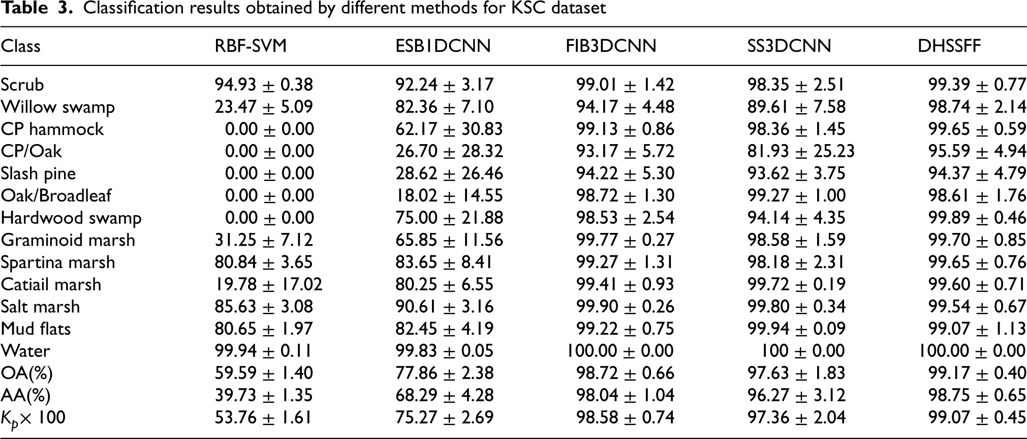
The classification results obtained through different methods for KSC dataset have been depicted in Table 3. We have reported the class-wise accuracy, OA, AA and Kp with standard deviation over 20 trials. The first 13 rows show the class wise accuracy and the last three rows represent OA, AA, and Kp. From the table, it can be observed that RBF-SVM performance is very poor for most of the classes. This is mainly happened due to the shallow learning nature of RBF-SVM. In particular, RBF-SVM fully misclassified few classes (CP hammock, CP/Oak, Slash pine, Oak/Broadleaf, Hardwood swamp) because of its inability in capturing the proper spectral information from limited training samples. Compared to RBF-SVM, EDB1DCNN shows better performance due to the deep feature extraction ability and has the support of spatial information. From the table, we can also see that all the spectral-spatial based methods such as FIB3DCNN, SS3DCNN, and DHSSFF have shown better classification results because of the combination of spectral and spatial information. Compared to FIB3DCNN and SS3DCNN, proposed DHSSFF has shown better classification result due to its deep feature fusion technique. With respect to class wise accuracy, DHSSFF obtained best classification accuracy in four classes (e.g. Scrub, Willow swamp, CP hammock and Spartina marsh) and marginally less in other classes among all the five methods. Moreover, DHSSFF has gained the improvement in OA by 0.45%, AA by 0.71% and Kp by 0.49% with its closest competitor FIB3DCNN.

Table 3

Classification results obtained by different methods for KSC dataset

Class	RBF-SVM	ESB1DCNN	FIB3DCNN	SS3DCNN	DHSSFF
Scrub	94.93 $\pm$ 0.38	92.24 $\pm$ 3.17	99.01 $\pm$ 1.42	98.35 $\pm$ 2.51	99.39 $\pm$ 0.77
Willow swamp	23.47 $\pm$ 5.09	82.36 $\pm$ 7.10	94.17 $\pm$ 4.48	89.61 $\pm$ 7.58	98.74 $\pm$ 2.14
CP hammock	0.00 $\pm$ 0.00	62.17 $\pm$ 30.83	99.13 $\pm$ 0.86	98.36 $\pm$ 1.45	99.65 $\pm$ 0.59
CP/Oak	0.00 $\pm$ 0.00	26.70 $\pm$ 28.32	93.17 $\pm$ 5.72	81.93 $\pm$ 25.23	95.59 $\pm$ 4.94
Slash pine	0.00 $\pm$ 0.00	28.62 $\pm$ 26.46	94.22 $\pm$ 5.30	93.62 $\pm$ 3.75	94.37 $\pm$ 4.79
Oak/Broadleaf	0.00 $\pm$ 0.00	18.02 $\pm$ 14.55	98.72 $\pm$ 1.30	99.27 $\pm$ 1.00	98.61 $\pm$ 1.76
Hardwood swamp	0.00 $\pm$ 0.00	75.00 $\pm$ 21.88	98.53 $\pm$ 2.54	94.14 $\pm$ 4.35	99.89 $\pm$ 0.46
Graminoid marsh	31.25 $\pm$ 7.12	65.85 $\pm$ 11.56	99.77 $\pm$ 0.27	98.58 $\pm$ 1.59	99.70 $\pm$ 0.85
Spartina marsh	80.84 $\pm$ 3.65	83.65 $\pm$ 8.41	99.27 $\pm$ 1.31	98.18 $\pm$ 2.31	99.65 $\pm$ 0.76
Catiail marsh	19.78 $\pm$ 17.02	80.25 $\pm$ 6.55	99.41 $\pm$ 0.93	99.72 $\pm$ 0.19	99.60 $\pm$ 0.71
Salt marsh	85.63 $\pm$ 3.08	90.61 $\pm$ 3.16	99.90 $\pm$ 0.26	99.80 $\pm$ 0.34	99.54 $\pm$ 0.67
Mud flats	80.65 $\pm$ 1.97	82.45 $\pm$ 4.19	99.22 $\pm$ 0.75	99.94 $\pm$ 0.09	99.07 $\pm$ 1.13
Water	99.94 $\pm$ 0.11	99.83 $\pm$ 0.05	100.00 $\pm$ 0.00	100 $\pm$ 0.00	100.00 $\pm$ 0.00
OA(%)	59.59 $\pm$ 1.40	77.86 $\pm$ 2.38	98.72 $\pm$ 0.66	97.63 $\pm$ 1.83	99.17 $\pm$ 0.40
AA(%)	39.73 $\pm$ 1.35	68.29 $\pm$ 4.28	98.04 $\pm$ 1.04	96.27 $\pm$ 3.12	98.75 $\pm$ 0.65
$K_{p} \times$ 100	53.76 $\pm$ 1.61	75.27 $\pm$ 2.69	98.58 $\pm$ 0.74	97.36 $\pm$ 2.04	99.07 $\pm$ 0.45

Fig. 6.

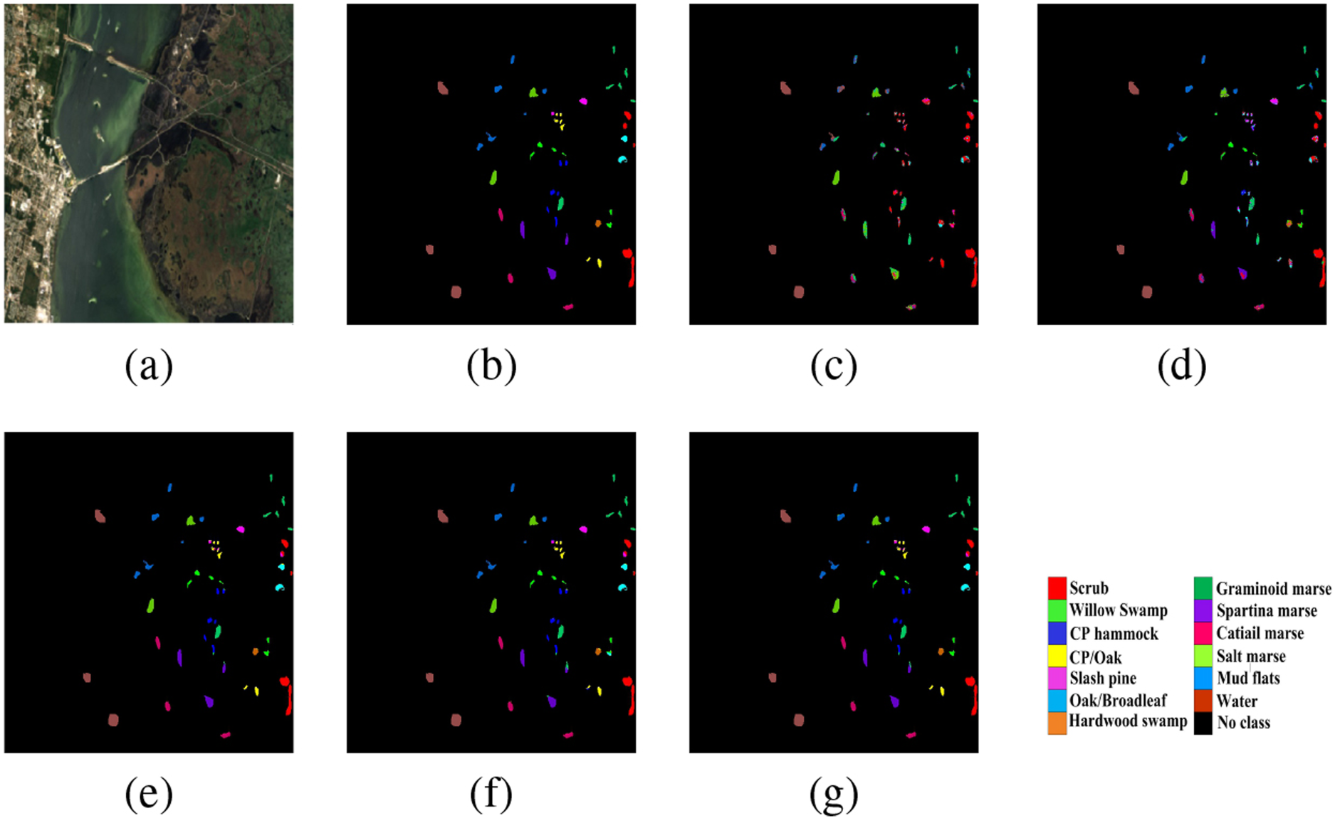
Classification maps for KSC dataset. (a) False color image (b) Ground truth. (c) RBF-SVM. (d) ESB1DCNN. (e) FIB3DCNN. (f) SS3DCNN. (g) DHSSFF.

Table 4

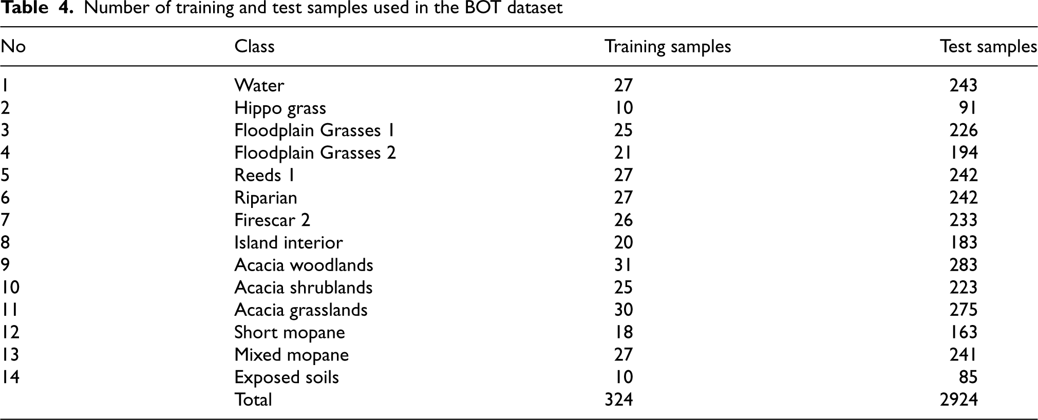
Number of training and test samples used in the BOT dataset

No	Class	Training samples	Test samples
1	Water	27	243
2	Hippo grass	10	91
3	Floodplain Grasses 1	25	226
4	Floodplain Grasses 2	21	194
5	Reeds 1	27	242
6	Riparian	27	242
7	Firescar 2	26	233
8	Island interior	20	183
9	Acacia woodlands	31	283
10	Acacia shrublands	25	223
11	Acacia grasslands	30	275
12	Short mopane	18	163
13	Mixed mopane	27	241
14	Exposed soils	10	85
	Total	324	2924

Apart from the quantitative evaluation, the classification maps have been generated using five methods on KSC dataset as shown in Fig. 6(c)–(g). It can be observed that RFB-SVM and ESB1DCNN could not generate accurate classification map due to utilization of spectral information only. The remaining methods have shown satisfactory performance, since they considered both spectral and spatial information.

3.5.2 Results on BOT dataset

In the BOT dataset, 10% samples from each class were randomly selected as training set and the rest samples were considered as test set. The distribution of training and test samples from each class are shown in Table 4.

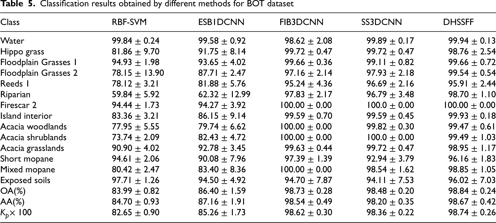
The classification results of five methods on BOT dataset have been shown in Table 5. From the table, we can see that all the spectral-spatial based methods including FIB3DCNN, SS3DCNN, and DHSSFF have shown better classification results than RBF-SVM and ESB1DCNN. In addition, the FIB3DCNN, SS3DCNN, and DHSSFF methods have achieved over 92% classification accuracy for all the classes and obtained absolutely correct classification results in the Firescar 2 class. However, many samples have been misclssified by RBF-SVM, ESB1DCNN, FIB3DCNN, and SS3DCNN in the Riparian class. Compared with these methods, DHSSFF has increased by 38.86%, 36.38%, 0.87%, and 1.91%, respectively. Beside this, DHSSFF has obtained high classification accuracy in most of the classes and achieved best statistical results in term of OA, AA, and $K_{p}$ .

Table 5
Classification results obtained by different methods for BOT dataset

Class RBF-SVM ESB1DCNN FIB3DCNN SS3DCNN DHSSFF

Water 99.84 $\pm$ 0.24 99.58 $\pm$ 0.92 98.62 $\pm$ 2.08 99.89 $\pm$ 0.17 99.94 $\pm$ 0.13

Hippo grass 81.86 $\pm$ 9.70 91.75 $\pm$ 8.14 99.72 $\pm$ 0.47 99.72 $\pm$ 0.47 98.76 $\pm$ 2.54

Floodplain Grasses 1 94.93 $\pm$ 1.98 93.65 $\pm$ 4.02 99.66 $\pm$ 0.36 99.11 $\pm$ 0.82 99.66 $\pm$ 0.72

Floodplain Grasses 2 78.15 $\pm$ 13.90 87.71 $\pm$ 2.47 97.16 $\pm$ 2.14 97.93 $\pm$ 2.18 99.54 $\pm$ 0.54

Reeds 1 78.12 $\pm$ 3.21 81.88 $\pm$ 5.76 95.24 $\pm$ 4.36 96.69 $\pm$ 2.16 95.91 $\pm$ 2.44

Riparian 59.84 $\pm$ 5.92 62.32 $\pm$ 12.99 97.83 $\pm$ 2.17 96.79 $\pm$ 3.48 98.70 $\pm$ 1.10

Firescar 2 94.44 $\pm$ 1.73 94.27 $\pm$ 3.92 100.00 $\pm$ 0.00 100.0 $\pm$ 0.00 100.00 $\pm$ 0.00

Island interior 83.36 $\pm$ 3.21 86.15 $\pm$ 9.14 99.59 $\pm$ 0.70 99.59 $\pm$ 0.45 99.93 $\pm$ 0.18

Acacia woodlands 77.95 $\pm$ 5.55 79.74 $\pm$ 6.62 100.00 $\pm$ 0.00 99.82 $\pm$ 0.30 99.47 $\pm$ 0.61

Acacia shrublands 73.74 $\pm$ 2.09 82.43 $\pm$ 4.72 100.00 $\pm$ 0.00 100.0 $\pm$ 0.00 99.49 $\pm$ 1.03

Acacia grasslands 90.90 $\pm$ 4.02 92.78 $\pm$ 3.45 99.63 $\pm$ 0.44 99.72 $\pm$ 0.47 98.95 $\pm$ 1.17

Short mopane 94.61 $\pm$ 2.06 90.08 $\pm$ 7.96 97.39 $\pm$ 1.39 92.94 $\pm$ 3.79 96.16 $\pm$ 1.83

Mixed mopane 80.42 $\pm$ 2.47 83.40 $\pm$ 8.36 100.00 $\pm$ 0.00 98.54 $\pm$ 1.62 98.85 $\pm$ 1.05

Exposed soils 97.71 $\pm$ 1.26 94.50 $\pm$ 4.92 94.70 $\pm$ 7.87 94.11 $\pm$ 7.53 96.02 $\pm$ 7.03

OA(%) 83.99 $\pm$ 0.82 86.40 $\pm$ 1.59 98.73 $\pm$ 0.28 98.48 $\pm$ 0.20 98.84 $\pm$ 0.24

AA(%) 84.70 $\pm$ 0.93 87.16 $\pm$ 1.91 98.54 $\pm$ 0.49 98.20 $\pm$ 0.35 98.67 $\pm$ 0.42

$K_{p}$ $\times$ 100 82.65 $\pm$ 0.90 85.26 $\pm$ 1.73 98.62 $\pm$ 0.30 98.36 $\pm$ 0.22 98.74 $\pm$ 0.26

Class	RBF-SVM	ESB1DCNN	FIB3DCNN	SS3DCNN	DHSSFF
Water	99.84 $\pm$ 0.24	99.58 $\pm$ 0.92	98.62 $\pm$ 2.08	99.89 $\pm$ 0.17	99.94 $\pm$ 0.13
Hippo grass	81.86 $\pm$ 9.70	91.75 $\pm$ 8.14	99.72 $\pm$ 0.47	99.72 $\pm$ 0.47	98.76 $\pm$ 2.54
Floodplain Grasses 1	94.93 $\pm$ 1.98	93.65 $\pm$ 4.02	99.66 $\pm$ 0.36	99.11 $\pm$ 0.82	99.66 $\pm$ 0.72
Floodplain Grasses 2	78.15 $\pm$ 13.90	87.71 $\pm$ 2.47	97.16 $\pm$ 2.14	97.93 $\pm$ 2.18	99.54 $\pm$ 0.54
Reeds 1	78.12 $\pm$ 3.21	81.88 $\pm$ 5.76	95.24 $\pm$ 4.36	96.69 $\pm$ 2.16	95.91 $\pm$ 2.44
Riparian	59.84 $\pm$ 5.92	62.32 $\pm$ 12.99	97.83 $\pm$ 2.17	96.79 $\pm$ 3.48	98.70 $\pm$ 1.10
Firescar 2	94.44 $\pm$ 1.73	94.27 $\pm$ 3.92	100.00 $\pm$ 0.00	100.0 $\pm$ 0.00	100.00 $\pm$ 0.00
Island interior	83.36 $\pm$ 3.21	86.15 $\pm$ 9.14	99.59 $\pm$ 0.70	99.59 $\pm$ 0.45	99.93 $\pm$ 0.18
Acacia woodlands	77.95 $\pm$ 5.55	79.74 $\pm$ 6.62	100.00 $\pm$ 0.00	99.82 $\pm$ 0.30	99.47 $\pm$ 0.61
Acacia shrublands	73.74 $\pm$ 2.09	82.43 $\pm$ 4.72	100.00 $\pm$ 0.00	100.0 $\pm$ 0.00	99.49 $\pm$ 1.03
Acacia grasslands	90.90 $\pm$ 4.02	92.78 $\pm$ 3.45	99.63 $\pm$ 0.44	99.72 $\pm$ 0.47	98.95 $\pm$ 1.17
Short mopane	94.61 $\pm$ 2.06	90.08 $\pm$ 7.96	97.39 $\pm$ 1.39	92.94 $\pm$ 3.79	96.16 $\pm$ 1.83
Mixed mopane	80.42 $\pm$ 2.47	83.40 $\pm$ 8.36	100.00 $\pm$ 0.00	98.54 $\pm$ 1.62	98.85 $\pm$ 1.05
Exposed soils	97.71 $\pm$ 1.26	94.50 $\pm$ 4.92	94.70 $\pm$ 7.87	94.11 $\pm$ 7.53	96.02 $\pm$ 7.03
OA(%)	83.99 $\pm$ 0.82	86.40 $\pm$ 1.59	98.73 $\pm$ 0.28	98.48 $\pm$ 0.20	98.84 $\pm$ 0.24
AA(%)	84.70 $\pm$ 0.93	87.16 $\pm$ 1.91	98.54 $\pm$ 0.49	98.20 $\pm$ 0.35	98.67 $\pm$ 0.42
$K_{p}$ $\times$ 100	82.65 $\pm$ 0.90	85.26 $\pm$ 1.73	98.62 $\pm$ 0.30	98.36 $\pm$ 0.22	98.74 $\pm$ 0.26

Figure 7 shows the classification maps of five methods on BOT dataset. As shown in Fig. 7(c)–(g), many samples belonging to the Floodplain Grasses 2, Reeds 1, Acacia woodlands, Acacia shrublands and Mixed mopane classes are misclassified by RBF-SVM and ESB1DCNN. Compared with them, FIB3DCNN, SS3DCNN and DHSSFF offer a better distinction among these classes. Compared with FIB3DCNN and SS3DCNN, DHSSFF has achieved better boundary localization in the Riparian class.

Fig. 7.

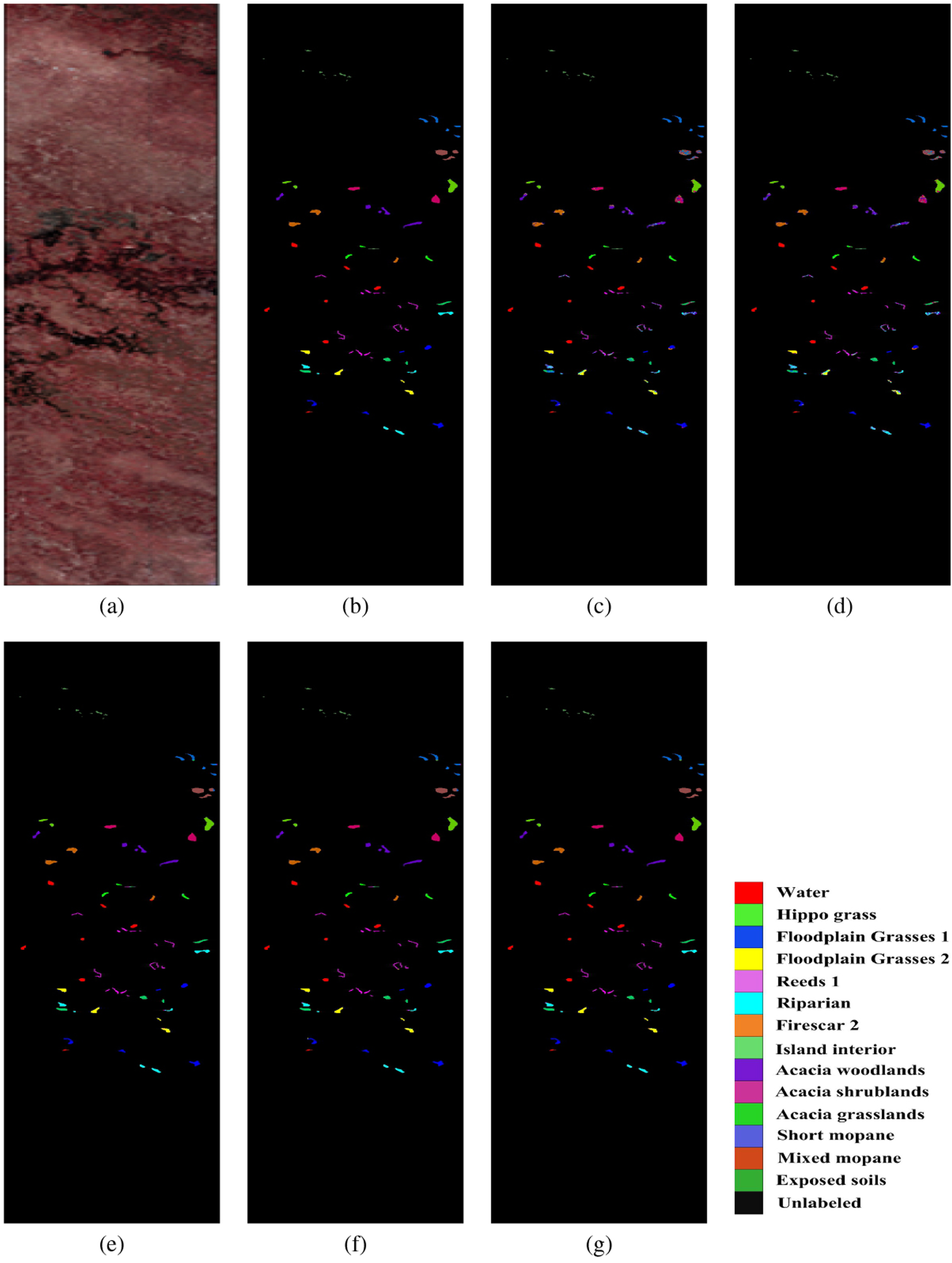
Classification maps for BOT dataset. (a) False color image. (b) Ground truth. (c) RBF-SVM. (d) ESB1DCNN. (e) FIB3DCNN. (f) SS3DCNN. (g) DHSSFF.

3.5.3 Results on IP dataset

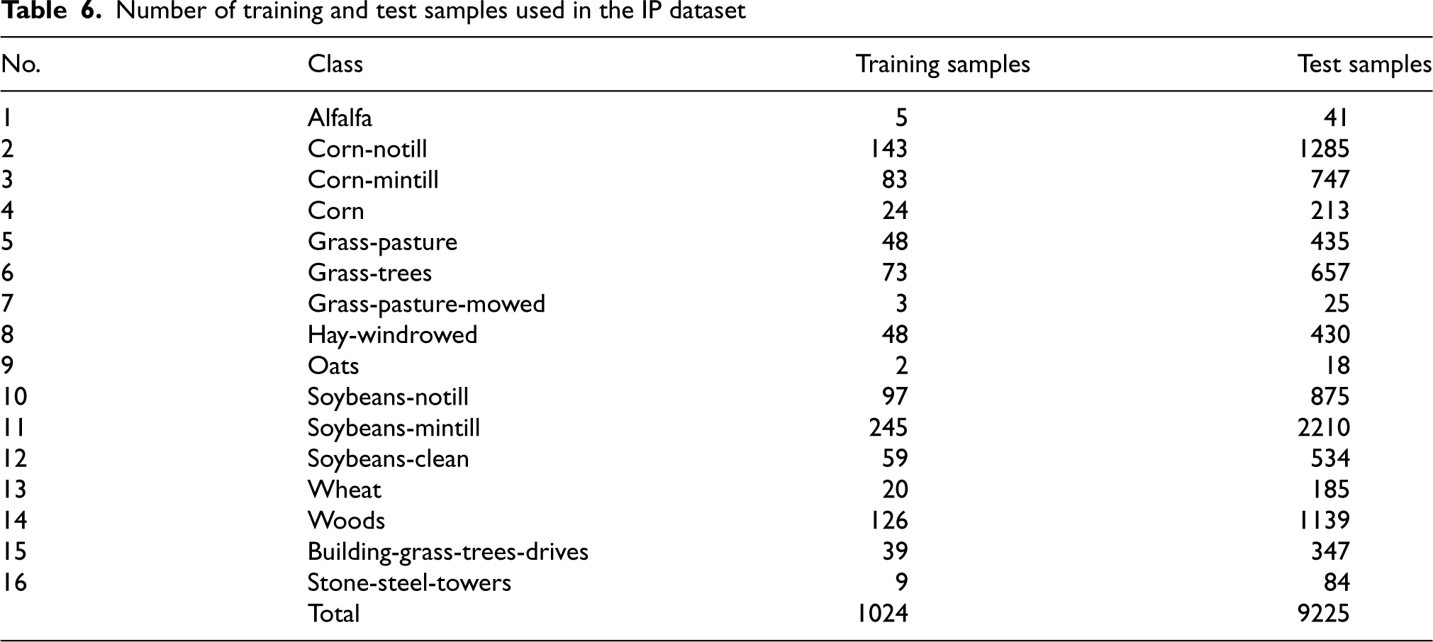
For IP dataset, 10% samples from each class were haphazardly selected as training set. The rest samples were considered as test set. The number of training and test samples from each class are listed in Table 6.

Table 6
Number of training and test samples used in the IP dataset

No. Class Training samples Test samples

1 Alfalfa 5 41

2 Corn-notill 143 1285

3 Corn-mintill 83 747

4 Corn 24 213

5 Grass-pasture 48 435

6 Grass-trees 73 657

7 Grass-pasture-mowed 3 25

8 Hay-windrowed 48 430

9 Oats 2 18

10 Soybeans-notill 97 875

11 Soybeans-mintill 245 2210

12 Soybeans-clean 59 534

13 Wheat 20 185

14 Woods 126 1139

15 Building-grass-trees-drives 39 347

16 Stone-steel-towers 9 84

Total 1024 9225

No.	Class	Training samples	Test samples
1	Alfalfa	5	41
2	Corn-notill	143	1285
3	Corn-mintill	83	747
4	Corn	24	213
5	Grass-pasture	48	435
6	Grass-trees	73	657
7	Grass-pasture-mowed	3	25
8	Hay-windrowed	48	430
9	Oats	2	18
10	Soybeans-notill	97	875
11	Soybeans-mintill	245	2210
12	Soybeans-clean	59	534
13	Wheat	20	185
14	Woods	126	1139
15	Building-grass-trees-drives	39	347
16	Stone-steel-towers	9	84
	Total	1024	9225

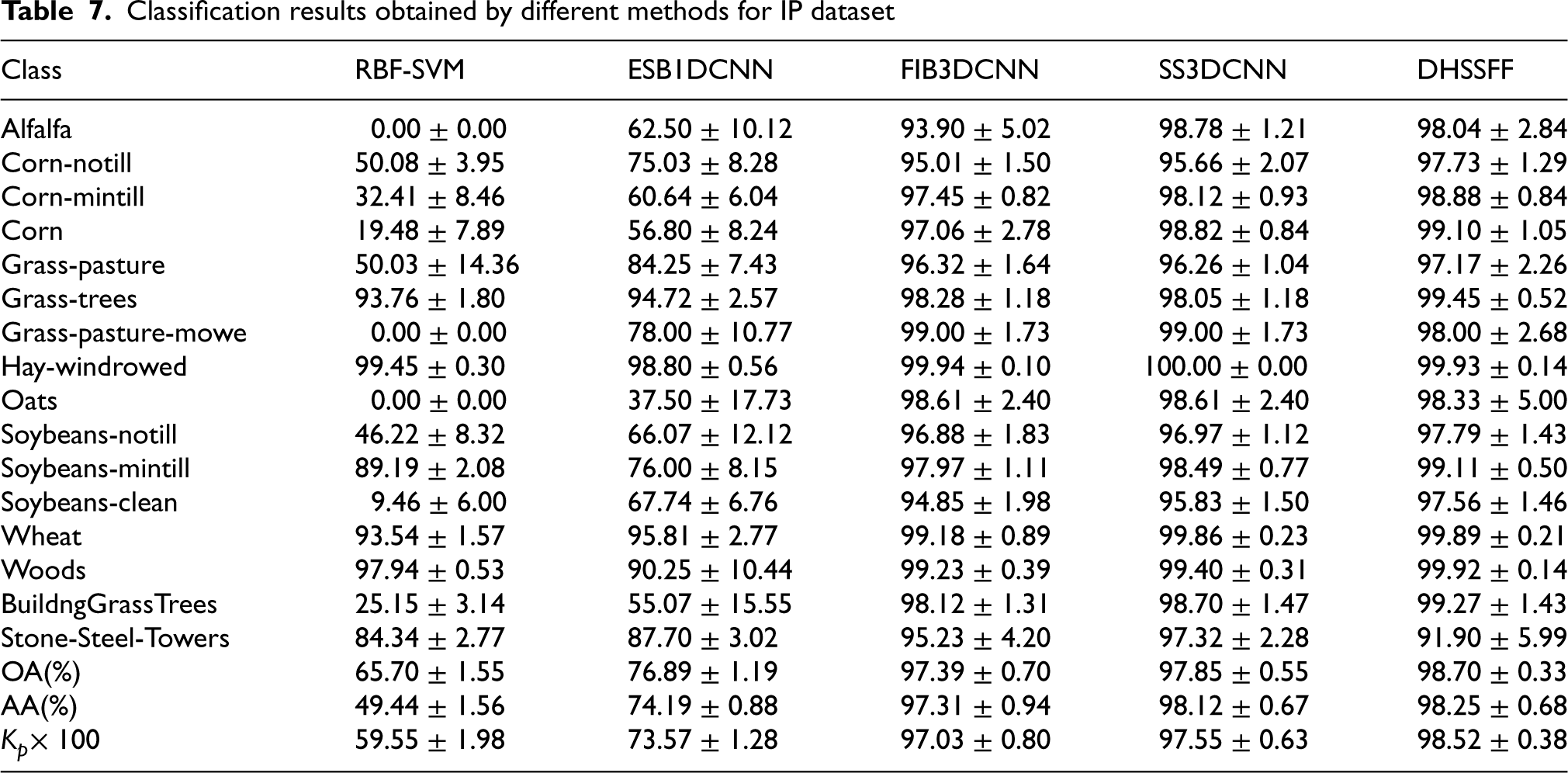
The classification performance of five methods for IP dataset has been shown in Table 7. It has been observed that most of the classes has achieved over 90% classification accuracy except RBF-SVM and ESB1DCNN. RBF-SVM has shown poor performance for most of the classes and totally failed to identify few classes (Alfalfa, Grass-pasture-mowe, Oats). This is occurred mainly due to the shallow learning nature of RBF-SVM and unable to handle the complex scene. Compared to RBF-SVM, ESB1DCNN has shown better results because of deep feature extraction ability. However, proposed DHSSFF has achieved the best class specific accuracies with low standard deviation on ten classes (namely Corn-notill, Corn-mintill, Corn, Grass-trees, Soybeans-notill, Soybeans-mintill, Soybeans-clean, Wheat, Woods and BuildngGrassTrees). Further, there is an improvement of 33%, 21.81%, 1.31%, and 0.85% in OA by DHSSFF compared with RBF-SVM, ESB1DCNN, FIB3DCNN and SS3DCNN, respectively.

The classification maps of IP dataset generated using five methods have been depicted in Fig. 8(c)–(g). Due to the absence of spatial features, RBF-SVM and ESB1DCNN suffers from misclassification of objects. On the contrary, other three methods take the advantage of spectral-spatial based features and yields better classification maps. It is worth nothing that compared with FIB3DCNN and SS3DCNN, the DHSSFF has achieved better clarity on Soybeans-mintill class.

Table 7

Classification results obtained by different methods for IP dataset

Class	RBF-SVM	ESB1DCNN	FIB3DCNN	SS3DCNN	DHSSFF
Alfalfa	0.00 $\pm$ 0.00	62.50 $\pm$ 10.12	93.90 $\pm$ 5.02	98.78 $\pm$ 1.21	98.04 $\pm$ 2.84
Corn-notill	50.08 $\pm$ 3.95	75.03 $\pm$ 8.28	95.01 $\pm$ 1.50	95.66 $\pm$ 2.07	97.73 $\pm$ 1.29
Corn-mintill	32.41 $\pm$ 8.46	60.64 $\pm$ 6.04	97.45 $\pm$ 0.82	98.12 $\pm$ 0.93	98.88 $\pm$ 0.84
Corn	19.48 $\pm$ 7.89	56.80 $\pm$ 8.24	97.06 $\pm$ 2.78	98.82 $\pm$ 0.84	99.10 $\pm$ 1.05
Grass-pasture	50.03 $\pm$ 14.36	84.25 $\pm$ 7.43	96.32 $\pm$ 1.64	96.26 $\pm$ 1.04	97.17 $\pm$ 2.26
Grass-trees	93.76 $\pm$ 1.80	94.72 $\pm$ 2.57	98.28 $\pm$ 1.18	98.05 $\pm$ 1.18	99.45 $\pm$ 0.52
Grass-pasture-mowe	0.00 $\pm$ 0.00	78.00 $\pm$ 10.77	99.00 $\pm$ 1.73	99.00 $\pm$ 1.73	98.00 $\pm$ 2.68
Hay-windrowed	99.45 $\pm$ 0.30	98.80 $\pm$ 0.56	99.94 $\pm$ 0.10	100.00 $\pm$ 0.00	99.93 $\pm$ 0.14
Oats	0.00 $\pm$ 0.00	37.50 $\pm$ 17.73	98.61 $\pm$ 2.40	98.61 $\pm$ 2.40	98.33 $\pm$ 5.00
Soybeans-notill	46.22 $\pm$ 8.32	66.07 $\pm$ 12.12	96.88 $\pm$ 1.83	96.97 $\pm$ 1.12	97.79 $\pm$ 1.43
Soybeans-mintill	89.19 $\pm$ 2.08	76.00 $\pm$ 8.15	97.97 $\pm$ 1.11	98.49 $\pm$ 0.77	99.11 $\pm$ 0.50
Soybeans-clean	9.46 $\pm$ 6.00	67.74 $\pm$ 6.76	94.85 $\pm$ 1.98	95.83 $\pm$ 1.50	97.56 $\pm$ 1.46
Wheat	93.54 $\pm$ 1.57	95.81 $\pm$ 2.77	99.18 $\pm$ 0.89	99.86 $\pm$ 0.23	99.89 $\pm$ 0.21
Woods	97.94 $\pm$ 0.53	90.25 $\pm$ 10.44	99.23 $\pm$ 0.39	99.40 $\pm$ 0.31	99.92 $\pm$ 0.14
BuildngGrassTrees	25.15 $\pm$ 3.14	55.07 $\pm$ 15.55	98.12 $\pm$ 1.31	98.70 $\pm$ 1.47	99.27 $\pm$ 1.43
Stone-Steel-Towers	84.34 $\pm$ 2.77	87.70 $\pm$ 3.02	95.23 $\pm$ 4.20	97.32 $\pm$ 2.28	91.90 $\pm$ 5.99
OA(%)	65.70 $\pm$ 1.55	76.89 $\pm$ 1.19	97.39 $\pm$ 0.70	97.85 $\pm$ 0.55	98.70 $\pm$ 0.33
AA(%)	49.44 $\pm$ 1.56	74.19 $\pm$ 0.88	97.31 $\pm$ 0.94	98.12 $\pm$ 0.67	98.25 $\pm$ 0.68
$K_{p}$ $\times$ 100	59.55 $\pm$ 1.98	73.57 $\pm$ 1.28	97.03 $\pm$ 0.80	97.55 $\pm$ 0.63	98.52 $\pm$ 0.38

Fig. 8.

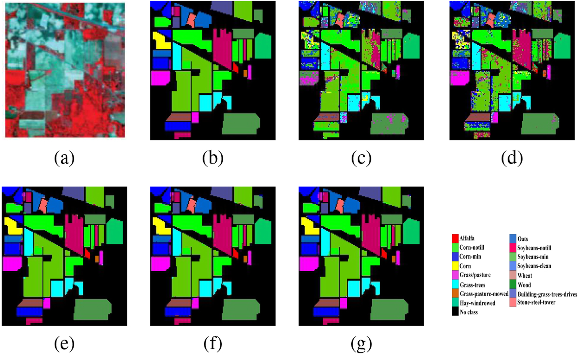
Classification maps for IP dataset. (a) False color image. (b) Ground truth. (c) RBF-SVM. (d) ESB1DCNN. (e) FIB3DCNN. (f) SS3DCNN. (g) DHSSFF.

3.5.4 Results on UP dataset

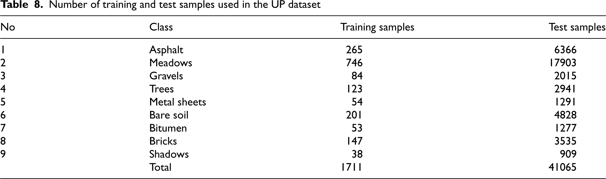
As abundant samples are available in UP dataset, only 4% samples from each class were haphazardly selected for training set and rest samples were considered for test set. The distribution of training and test samples from each class are depicted in Table 8.

Table 8
Number of training and test samples used in the UP dataset

No Class Training samples Test samples

1 Asphalt 265 6366

2 Meadows 746 17903

3 Gravels 84 2015

4 Trees 123 2941

5 Metal sheets 54 1291

6 Bare soil 201 4828

7 Bitumen 53 1277

8 Bricks 147 3535

9 Shadows 38 909

Total 1711 41065

No	Class	Training samples	Test samples
1	Asphalt	265	6366
2	Meadows	746	17903
3	Gravels	84	2015
4	Trees	123	2941
5	Metal sheets	54	1291
6	Bare soil	201	4828
7	Bitumen	53	1277
8	Bricks	147	3535
9	Shadows	38	909
	Total	1711	41065

Table 9

Classification results obtained by different methods for UP dataset

Classe	RBF-SVM	ESB1DCNN	FIB3DCNN	SS3DCNN	DHSSFF
Asphalt	91.35 $\pm$ 0.46	88.95 $\pm$ 1.83	98.89 $\pm$ 0.29	98.94 $\pm$ 0.95	99.22 $\pm$ 0.39
Meadows	98.80 $\pm$ 0.80	92.08 $\pm$ 2.06	99.94 $\pm$ 0.03	99.88 $\pm$ 0.05	99.95 $\pm$ 0.05
Gravels	0.28 $\pm$ 0.47	53.90 $\pm$ 11.75	97.75 $\pm$ 0.75	96.48 $\pm$ 1.53	97.07 $\pm$ 1.08
Trees	73.02 $\pm$ 3.05	82.97 $\pm$ 6.09	96.28 $\pm$ 0.87	97.35 $\pm$ 0.87	97.03 $\pm$ 0.80
Metal Sheets	99.22 $\pm$ 0.19	99.58 $\pm$ 0.20	99.45 $\pm$ 0.56	99.59 $\pm$ 0.41	99.75 $\pm$ 0.36
Bare soil	15.70 $\pm$ 3.06	52.24 $\pm$ 5.29	99.76 $\pm$ 0.23	97.16 $\pm$ 0.05	99.71 $\pm$ 0.20
Bitumen	0.00 $\pm$ 0.00	36.82 $\pm$ 16.50	97.08 $\pm$ 1.28	96.65 $\pm$ 2.36	97.79 $\pm$ 1.27
Bricks	93.59 $\pm$ 0.92	87.54 $\pm$ 5.67	98.34 $\pm$ 0.68	96.85 $\pm$ 4.42	98.80 $\pm$ 0.63
Shadows	99.79 $\pm$ 0.10	99.82 $\pm$ 0.05	93.89 $\pm$ 1.61	96.79 $\pm$ 2.00	95.22 $\pm$ 3.03
OA(%)	77.27 $\pm$ 0.36	82.68 $\pm$ 0.97	99.01 $\pm$ 0.12	98.81 $\pm$ 0.60	99.18 $\pm$ 0.14
AA(%)	63.42 $\pm$ 0.50	77.10 $\pm$ 2.27	97.93 $\pm$ 0.26	97.75 $\pm$ 0.85	98.28 $\pm$ 0.43
$K_{p} \times$ 100	68.14 $\pm$ 0.55	76.68 $\pm$ 1.29	98.69 $\pm$ 0.16	98.43 $\pm$ 0.80	98.92 $\pm$ 0.18

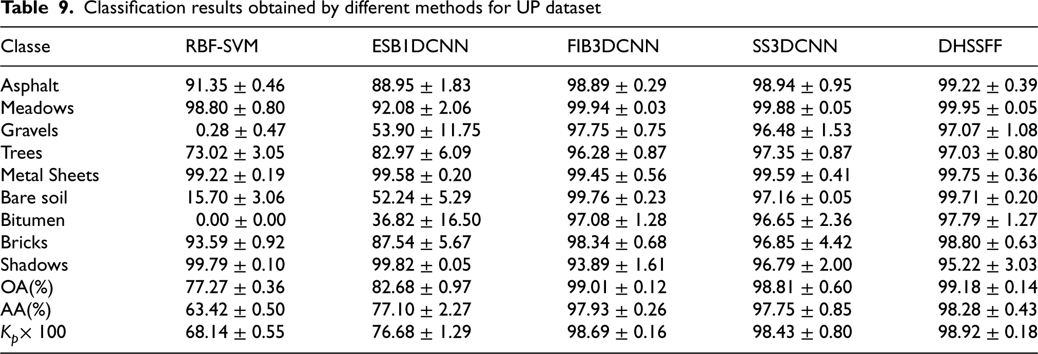
The classification performance using five methods on UP dataset have been presented in Table 9. From the table, we can observe that RBF-SVM has shown unsatisfactory results for Gravels and Bitumen classes. However, it is found that the quantitative assessment of FIB3DCNN, SS3DCNN and DHSSFF are superior than RBF-SVM, and ESB1DCNN by almost 16% on the basis of OA. Nevertheless, less than 1% difference was found in OA among spectral-spatial based methods. Further, the DHSSFF has achieved over 97% classification accuracy for all the classes except Shadows class. In addition, DHSSFF model is able to obtain almost correct classification results in asphalt, meadows, metal sheets, and bare soils classes.

Figure 9 shows the classification maps generated using five methods on UP dataset. As shown in Fig. 9(c) and 9(d), many samples belonging to the Bitumen class are misclassified as the Asphalt class by RBF-SVM and ESB1DCNN due to similar spectral characteristic. Similarly, RBF-SVM and ESB1DCNN misclassified many samples belonging to the Bare soil class due to the lack of spatial information. Compared with them, FIB3DCNN, SS3DCNN and DHSSFF have shown finer regional clarity in the bare soil class. Moreover, DHSSFF has gained improved boundary appearance in the Bitumen class.

Fig. 9.

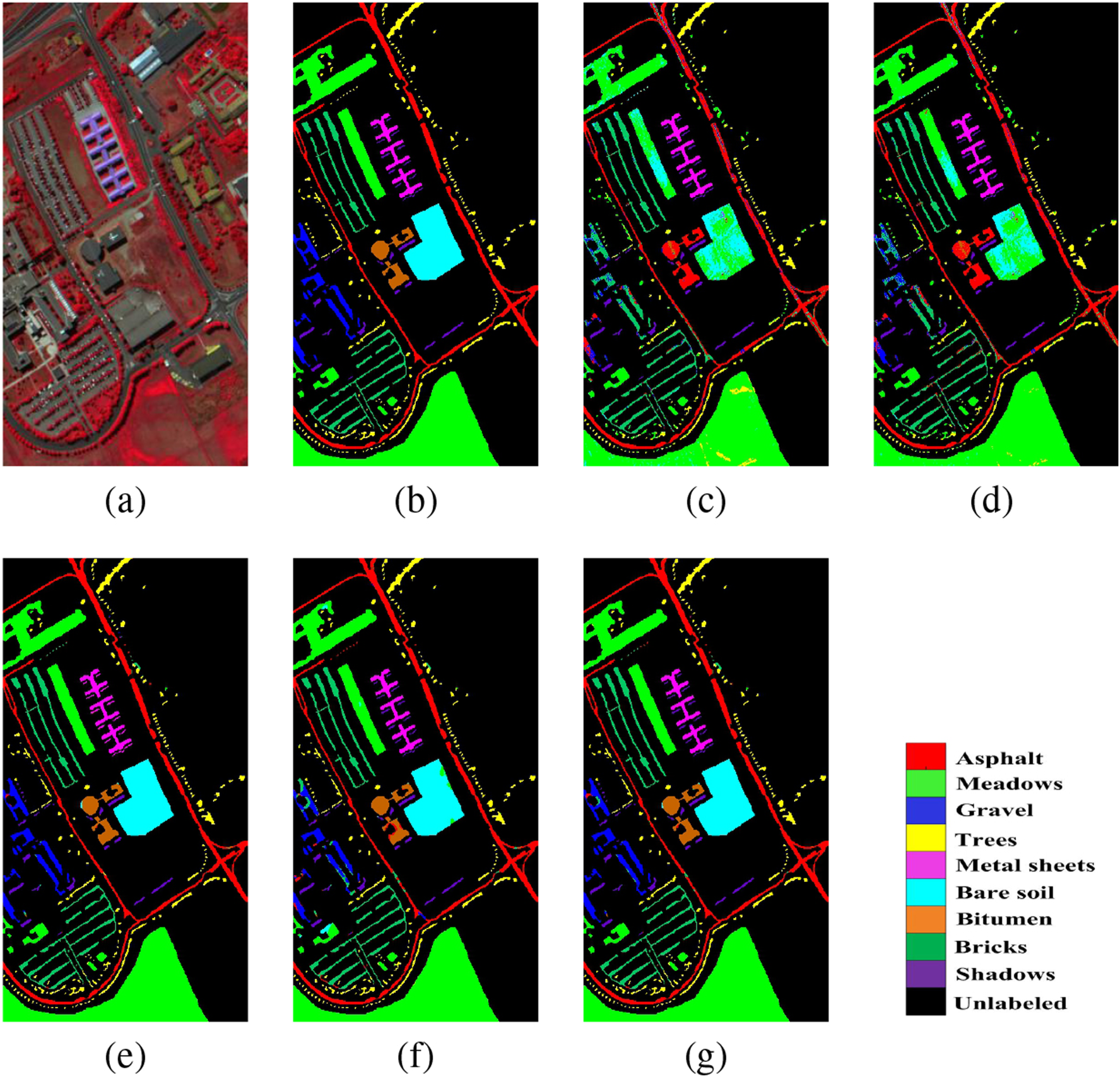
Classification maps for UP dataset. (a) False color image. (b) Ground truth. (c) RBF-SVM. (d) ESB1DCNN. (e) FIB3DCNN. (f) SS3DCNN. (g) DHSSFF.

3.5.5 Results on SA dataset

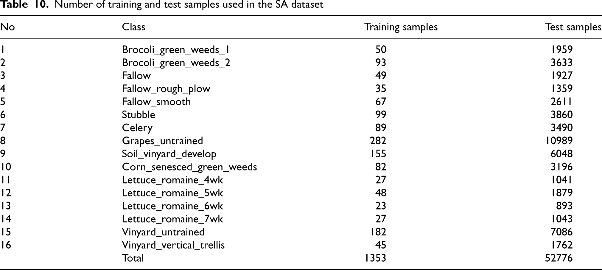
For SA dataset, only 2.5% samples from each class were randomly selected for training and rest samples were considered for testing. The number of training and test samples from each class are listed in Table 10.

Table 10
Number of training and test samples used in the SA dataset

No Class Training samples Test samples

1 Brocoli_green_weeds_1 50 1959

2 Brocoli_green_weeds_2 93 3633

3 Fallow 49 1927

4 Fallow_rough_plow 35 1359

5 Fallow_smooth 67 2611

6 Stubble 99 3860

7 Celery 89 3490

8 Grapes_untrained 282 10989

9 Soil_vinyard_develop 155 6048

10 Corn_senesced_green_weeds 82 3196

11 Lettuce_romaine_4wk 27 1041

12 Lettuce_romaine_5wk 48 1879

13 Lettuce_romaine_6wk 23 893

14 Lettuce_romaine_7wk 27 1043

15 Vinyard_untrained 182 7086

16 Vinyard_vertical_trellis 45 1762

Total 1353 52776

No	Class	Training samples	Test samples
1	Brocoli_green_weeds_1	50	1959
2	Brocoli_green_weeds_2	93	3633
3	Fallow	49	1927
4	Fallow_rough_plow	35	1359
5	Fallow_smooth	67	2611
6	Stubble	99	3860
7	Celery	89	3490
8	Grapes_untrained	282	10989
9	Soil_vinyard_develop	155	6048
10	Corn_senesced_green_weeds	82	3196
11	Lettuce_romaine_4wk	27	1041
12	Lettuce_romaine_5wk	48	1879
13	Lettuce_romaine_6wk	23	893
14	Lettuce_romaine_7wk	27	1043
15	Vinyard_untrained	182	7086
16	Vinyard_vertical_trellis	45	1762
	Total	1353	52776

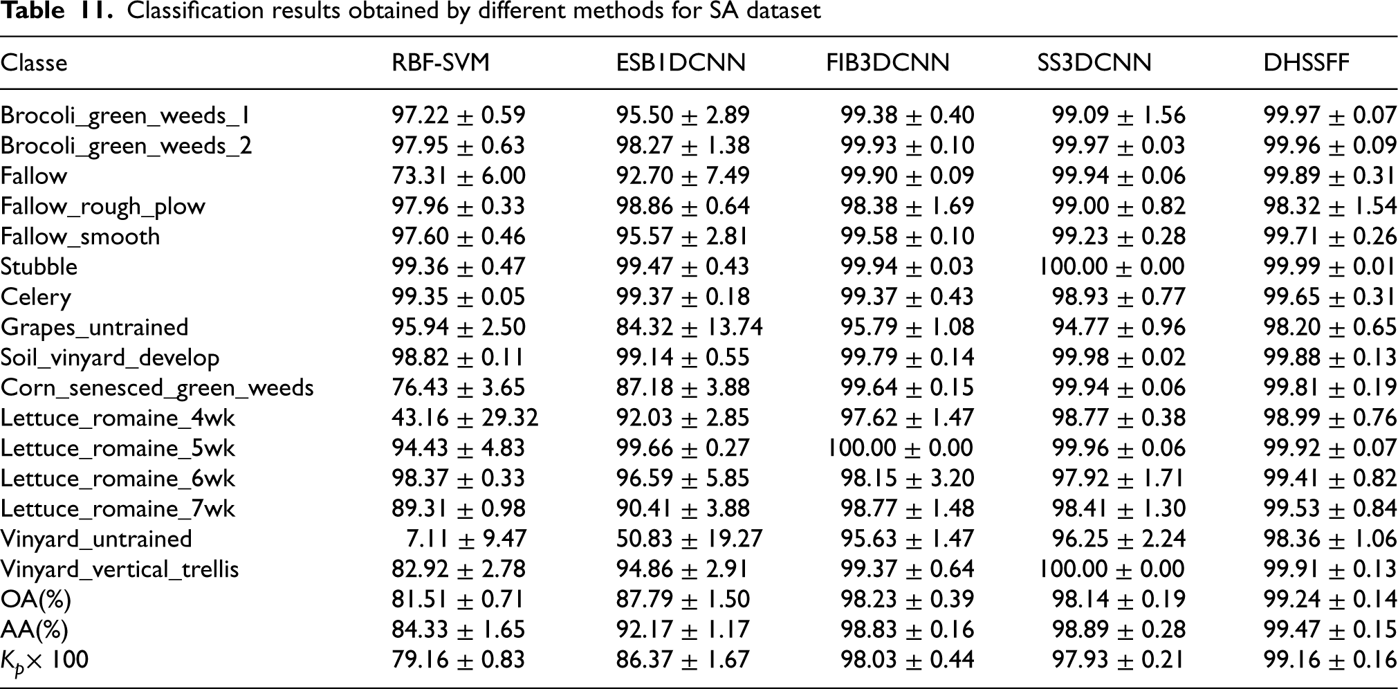
The classification results of five methods on SA dataset have been shown in Table 11. It can be seen that more than 92% classification accuracy has been obtained for most of the classes using all five methods. However, for grapes_untrained class, the classification results of FIB3DCNN and SS3DCNN are not satisfactory but DHSSFF has shown improvement in OA by 2.31% and 3.5%, respectively. Again, DHSSFF has increased 2.73% and 2.11%, respectively, for Vinyard_untrained class. Further, compared with FIB3DCNN and SS3DCNN, DHSSFF increases about 1.13% and 1.23%, respectively, in terms of $K_{p}$ . This kind of improvement is happened mainly due to the effective deep feature fusion of DHSSFF. With respect to OA, AA, and $K_{p}$ , DHSSFF has outperformed amongst five methods.

Figure 10(c)–(g) shows the classification maps generated using five methods on SA dataset. It can be observed that FIB3DCNN, SS3DCNN and DHSSFF provided better classification maps than RBF-SVM and ESB1DCNN. For instance, several samples of grapes_untrained and vinyard_untrained class have been misclassified by RBF-SVM and ESB1DCNN which leads to fuzzy classification maps. Comparing with FIB3DCNN, and SS3DCNN, our proposed model DHSSFF provided a better distinction between these two classes by removing noisy scatter points. In addition, DHSSFF has shown improved boundary localization in the Brocoli_green_weeds_1 class.

Table 11

Classification results obtained by different methods for SA dataset

Classe	RBF-SVM	ESB1DCNN	FIB3DCNN	SS3DCNN	DHSSFF
Brocoli_green_weeds_1	97.22 $\pm$ 0.59	95.50 $\pm$ 2.89	99.38 $\pm$ 0.40	99.09 $\pm$ 1.56	99.97 $\pm$ 0.07
Brocoli_green_weeds_2	97.95 $\pm$ 0.63	98.27 $\pm$ 1.38	99.93 $\pm$ 0.10	99.97 $\pm$ 0.03	99.96 $\pm$ 0.09
Fallow	73.31 $\pm$ 6.00	92.70 $\pm$ 7.49	99.90 $\pm$ 0.09	99.94 $\pm$ 0.06	99.89 $\pm$ 0.31
Fallow_rough_plow	97.96 $\pm$ 0.33	98.86 $\pm$ 0.64	98.38 $\pm$ 1.69	99.00 $\pm$ 0.82	98.32 $\pm$ 1.54
Fallow_smooth	97.60 $\pm$ 0.46	95.57 $\pm$ 2.81	99.58 $\pm$ 0.10	99.23 $\pm$ 0.28	99.71 $\pm$ 0.26
Stubble	99.36 $\pm$ 0.47	99.47 $\pm$ 0.43	99.94 $\pm$ 0.03	100.00 $\pm$ 0.00	99.99 $\pm$ 0.01
Celery	99.35 $\pm$ 0.05	99.37 $\pm$ 0.18	99.37 $\pm$ 0.43	98.93 $\pm$ 0.77	99.65 $\pm$ 0.31
Grapes_untrained	95.94 $\pm$ 2.50	84.32 $\pm$ 13.74	95.79 $\pm$ 1.08	94.77 $\pm$ 0.96	98.20 $\pm$ 0.65
Soil_vinyard_develop	98.82 $\pm$ 0.11	99.14 $\pm$ 0.55	99.79 $\pm$ 0.14	99.98 $\pm$ 0.02	99.88 $\pm$ 0.13
Corn_senesced_green_weeds	76.43 $\pm$ 3.65	87.18 $\pm$ 3.88	99.64 $\pm$ 0.15	99.94 $\pm$ 0.06	99.81 $\pm$ 0.19
Lettuce_romaine_4wk	43.16 $\pm$ 29.32	92.03 $\pm$ 2.85	97.62 $\pm$ 1.47	98.77 $\pm$ 0.38	98.99 $\pm$ 0.76
Lettuce_romaine_5wk	94.43 $\pm$ 4.83	99.66 $\pm$ 0.27	100.00 $\pm$ 0.00	99.96 $\pm$ 0.06	99.92 $\pm$ 0.07
Lettuce_romaine_6wk	98.37 $\pm$ 0.33	96.59 $\pm$ 5.85	98.15 $\pm$ 3.20	97.92 $\pm$ 1.71	99.41 $\pm$ 0.82
Lettuce_romaine_7wk	89.31 $\pm$ 0.98	90.41 $\pm$ 3.88	98.77 $\pm$ 1.48	98.41 $\pm$ 1.30	99.53 $\pm$ 0.84
Vinyard_untrained	7.11 $\pm$ 9.47	50.83 $\pm$ 19.27	95.63 $\pm$ 1.47	96.25 $\pm$ 2.24	98.36 $\pm$ 1.06
Vinyard_vertical_trellis	82.92 $\pm$ 2.78	94.86 $\pm$ 2.91	99.37 $\pm$ 0.64	100.00 $\pm$ 0.00	99.91 $\pm$ 0.13
OA(%)	81.51 $\pm$ 0.71	87.79 $\pm$ 1.50	98.23 $\pm$ 0.39	98.14 $\pm$ 0.19	99.24 $\pm$ 0.14
AA(%)	84.33 $\pm$ 1.65	92.17 $\pm$ 1.17	98.83 $\pm$ 0.16	98.89 $\pm$ 0.28	99.47 $\pm$ 0.15
$K_{p} \times$ 100	79.16 $\pm$ 0.83	86.37 $\pm$ 1.67	98.03 $\pm$ 0.44	97.93 $\pm$ 0.21	99.16 $\pm$ 0.16

Fig. 10.

Classification maps for SA dataset. (a) False color image. (b) Ground truth. (c) RBF-SVM. (d) ESB1DCNN. (e) FIB3DCNN. (f) SS3DCNN. (g) DHSSFF.

Table 12

Performance comparison of different fusion methods (dash (-) indicates data not available)

	CSFF [33]			MLFFSA [47]			FFUN [31]			UMF [38]			DHSSFF
Dataset	OA	AA	$K_{p}$	OA	AA	$K_{p}$	OA	AA	$K_{p}$	OA	AA	$K_{p}$	OA	AA	$K_{p}$
KSC	–	–	–	–	–	–	97.71	–	97.45	97.79	97.73	97.54	99.17	98.75	99.07
BOT	–	–	–	–	–	–	–	–	–	–	–	–	98.84	98.67	98.74
IP	98.65	99.22	–	98.2	94.4	97.9	98.40	–	98.14	97.24	96.93	96.85	98.70	98.25	98.52
UP	97.50	94.63	–	99.1	98.1	98.9	99.46	–	99.26	94.12	95.38	92.33	99.18	98.28	98.92
SA	–	–	–	98.7	98.7	98.6	–	–	–	95.38	97.17	94.87	99.24	99.47	99.16

Table 13

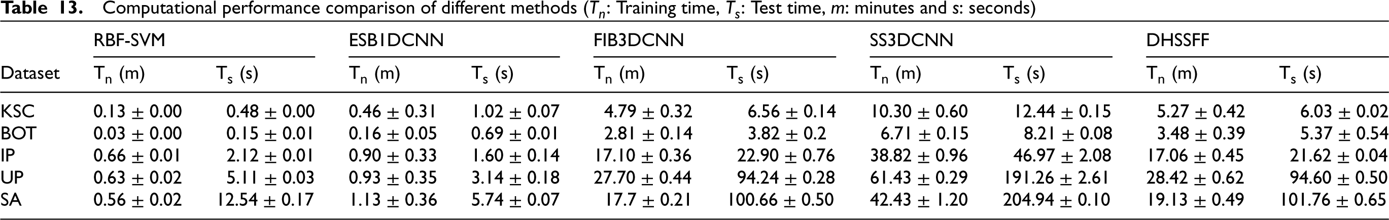
Computational performance comparison of different methods ( $T_{n}$ : Training time, $T_{s}$ : Test time, $m$ : minutes and $s$ : seconds)

	RBF-SVM		ESB1DCNN		FIB3DCNN		SS3DCNN		DHSSFF
Dataset	T_n (m)	T_s (s)	T_n (m)	T_s (s)	T_n (m)	T_s (s)	T_n (m)	T_s (s)	T_n (m)	T_s (s)
KSC	0.13 $\pm$ 0.00	0.48 $\pm$ 0.00	0.46 $\pm$ 0.31	1.02 $\pm$ 0.07	4.79 $\pm$ 0.32	6.56 $\pm$ 0.14	10.30 $\pm$ 0.60	12.44 $\pm$ 0.15	5.27 $\pm$ 0.42	6.03 $\pm$ 0.02
BOT	0.03 $\pm$ 0.00	0.15 $\pm$ 0.01	0.16 $\pm$ 0.05	0.69 $\pm$ 0.01	2.81 $\pm$ 0.14	3.82 $\pm$ 0.2	6.71 $\pm$ 0.15	8.21 $\pm$ 0.08	3.48 $\pm$ 0.39	5.37 $\pm$ 0.54
IP	0.66 $\pm$ 0.01	2.12 $\pm$ 0.01	0.90 $\pm$ 0.33	1.60 $\pm$ 0.14	17.10 $\pm$ 0.36	22.90 $\pm$ 0.76	38.82 $\pm$ 0.96	46.97 $\pm$ 2.08	17.06 $\pm$ 0.45	21.62 $\pm$ 0.04
UP	0.63 $\pm$ 0.02	5.11 $\pm$ 0.03	0.93 $\pm$ 0.35	3.14 $\pm$ 0.18	27.70 $\pm$ 0.44	94.24 $\pm$ 0.28	61.43 $\pm$ 0.29	191.26 $\pm$ 2.61	28.42 $\pm$ 0.62	94.60 $\pm$ 0.50
SA	0.56 $\pm$ 0.02	12.54 $\pm$ 0.17	1.13 $\pm$ 0.36	5.74 $\pm$ 0.07	17.7 $\pm$ 0.21	100.66 $\pm$ 0.50	42.43 $\pm$ 1.20	204.94 $\pm$ 0.10	19.13 $\pm$ 0.49	101.76 $\pm$ 0.65

3.6 Benchmarking with fusion models

In this paper, we fused deep spectral and spatial features to explore the discriminative information existing in deep architecture. In literature, various fusion based deep learning models have been proposed for HSI classification. To show the effectiveness of our DHSSFF model, the classification results of different fusion based models on HSI datasets have been reported in Table 12.

The following methods have been considered for comparison: class-specific feature fusion (CSFF) [33], multilayer feature fusion and sample augmentation (MLFFSA) [47], feature fusion through unified network (FFUN) [31], and unsupervised method for fusion (UMF) [38]. CSFF utilized stacked denoising autoencoder, and CNN as a feature extraction tools for spectral, and spatial information, respectively before applying fusion scheme. MLFFFSA exploited multilayer feature fusion for extracting complementary information among sallow and deep layers. Further, a band grouping oriented long short-term memory and a CNN architecture has been applied in FFUN for spectral and spatial feature extraction, respectively. Another fusion model, UMF extracted multiscale deep spatial feature by utilizing pre-trained filter banks in VGG16 and fused spectral and spatial features through unsupervised cooperative sparse autoencoder.

From Table 12, we can observed that the FFUN and UMF methods have been reported OA as 97.71% and 97.79% respectively, which is 1.46% and 1.38% lower than our proposed model on KSC dataset. Compared with FFUN and UMF, DHSSFF shows better classification performance because of effective deep spectral-spatial feature fusion scheme. In case of IP dataset, the proposed model obtains marginally higher OA with 0.05%, 0.5%, 0.3%, and 1.46% improvement over CSFF, MLFFSA, FFUN, and UMF method, respectively. Here, compared with CSFF, MLFFSA, FFUN, and UMF models, DHSSFF has shown superior performance in term of OA for most of the cases on UP, and SA datasets.

3.7 Analysis of the computational complexity

In this section, we have explained the running time of various methods for HSI classification. The detailed information of training time (for 200 epochs) and test time of five methods on KSC, BOT, IP, UP, and SA datasets have been provided in Table 13. It can be seen that RBF-SVM and ESB1DCNN are much faster during training than FIB3DCNN, SS3DCNN, and DHSSFF but failed to show better classification results due to the simple architecture. As other three methods are based on 3D CNN architecture, they require more time to tune large number of parameters. Among these three methods, SS3DCNN consumed more time on training because of the involvement of regularization technique. In case of FIB3DCNN and DHFFSS methods, the training time is almost similar but DHFFSS method is able to achieve better classification accuracy for all aforementioned datasets.

Although, all the spectral-spatial based methods consume long time to train the model, the test time is much smaller compared with the training time. Moreover, the test time has a positive correlation with number of samples in a test set. The proposed method took an average of 6 seconds, 5 seconds, 21 seconds, 94 seconds, and 101 seconds for 4690, 2924, 9225, 41065, and 52776 test samples on KSC, BOT, IP, UP, and SA datasets, respectively. This demonstrates that our proposed method is capable to reach high classification accuracy with acceptable computational time.

4. Conclusion

In this paper, we have proposed a simple yet quite effective novel CNN based two-channel model with spectral-spatial feature fusion for HSI classification. In our model, the 1D CNN as first channel is adopted to exploit the spectral features by considering entire spectral bands of HSI whereas 3D CNN as second channel is employed to extract deep spatial features by selecting few informative bands of HSI. In the fusion stage, the deep features from two channels were concatenated, which learns the discriminative spectral and spatial information fully and effectively. In our experiments, five widely used HSI datasets were utilized to evaluate the effectiveness of separate feature extarction and fusion technique. Experimental results demonstrate that the standalone 3D CNN demonstrates high performance across all five datasets. However, DHSSFF, a fusion model incorporating both 1D CNN and 3D CNN, enhances performance with only a marginal rise in computational cost. Consequently, we can conclude that the proposed DHSSFF model can efficiently extract the deep features from two channels and fuse them properly. With the help of separate feature extraction and fusion technique, DHSSFF shown competitive performance compared with state-of-the-art methods.

In future, we intend to resolve the sample imbalance issue and misclassification problem at boundary regions. However, training time of the proposed model is slightly more. Therefore, further research will be conducted on more efficient computational scheme. Moreover, we will concentrate on improving the performance of the proposed model by incorporating fusion scheme at feature extraction stage.

Footnotes

Acknowledgements

The authors extend their appreciation to the Deanship of Research and Graduate Studies at King Khalid University for funding this work through the Large Research Project.

Availability statement

The data presented in this article are publicly available in github repository, [https://github.com/eecn/ Hyperspectral-Classification].

References

Wilkinson

, A review of current issues in the integration of GIS and remote sensing data, International Journal of Geographical Information Science 10(1) (1996), 85–101.

Grewal

Kasana

S.S.

Kasana

, Hyperspectral image segmentation: a comprehensive survey, Multimedia Tools and Applications 82(14) (2023), 20819–20872.

Makki

Younes

Francis

Bianchi

Zucchetti

, A survey of landmine detection using hyperspectral imaging, ISPRS Journal of Photogrammetry and Remote Sensing 124 (2017), 40–53.

Rhee

Carbone

G.J.

, Monitoring agricultural drought for arid and humid regions using multi-sensor remote sensing data, Remote Sensing of Environment 114(12) (2010), 2875–2887.

Lin

Yan

, A support vector machine classifier based on a new kernel function model for hyperspectral data, GIScience & Remote Sensing 53(1) (2016), 85–101.

Liu

Choo

K.-K.R.

Wang

Huang

, SVM or deep learning? A comparative study on remote sensing image classification, Soft Computing 21(23) (2017), 7053–7065.

Huang

Zhang

Pižurica

, A robust sparse representation model for hyperspectral image classification, Sensors 17(9) (2017), 2087.

Pradhan

M.K.

Minz

Shrivastava

V.K.

, A Kernel-Based Extreme Learning Machine Framework for Classification of Hyperspectral Images Using Active Learning, Journal of the Indian Society of Remote Sensing 47(10) (2019), 1693–1705.

Chen

Lin

Zhao

Wang

, Deep learning-based classification of hyperspectral data, IEEE Journal of Selected Topics in Applied Earth Observations and Remote Sensing 7(6) (2014), 2094–2107.

10.

Zhao

, Spectral–spatial feature extraction for hyperspectral image classification: A dimension reduction and deep learning approach, IEEE Transactions on Geoscience and Remote Sensing 54(8) (2016), 4544–4554.

11.

Fauvel

Benediktsson

J.A.

Chanussot

Sveinsson

J.R.

, Spectral and spatial classification of hyperspectral data using SVMs and morphological profiles, IEEE Transactions on Geoscience and Remote Sensing 46(11) (2008), 3804–3814.

12.

Cao

Wang

Jiao

Han

, Fast hyperspectral band selection based on spatial feature extraction, Journal of Real-Time Image Processing 15(3) (2018), 555–564.

13.

Zhang

Wang

Zhang

Fei

, Adaptive total variation-based spectral-spatial feature extraction of hyperspectral image, Journal of Visual Communication and Image Representation 56 (2018), 150–159.

14.

Chen

Zhao

Jia

, Spectral–spatial classification of hyperspectral data based on deep belief network, IEEE Journal of Selected Topics in Applied Earth Observations and Remote Sensing 8(6) (2015), 2381–2392.

15.

Krizhevsky

Sutskever

Hinton

G.E.

, Imagenet classification with deep convolutional neural networks, in: Advances in neural information processing systems, 2012, pp. 1097–1105.

16.

Ignatov

, Real-time human activity recognition from accelerometer data using Convolutional Neural Networks, Applied Soft Computing 62 (2018), 915–922.

17.

Tang

Lin

Schmidt

Wang

Guo

Liang

, An eye detection method based on convolutional neural networks and support vector machines, Intelligent Data Analysis 22(2) (2018), 345–362.

18.

Karthick

Samuel

D.J.

Prakash

Sathyaprakash

Daruvuri

Ali

M.H.

Aiswarya

, Real-time MRI lungs images revealing using Hybrid feedforward Deep Neural Network and Convolutional Neural Network, Intelligent Data Analysis (2023), 1–20.

19.

Bilal

Munawar

Shaikh

M.S.

Al-Saggaf

U.M.

Kada

, Hyperspectral Image Segmentation using End-to-End CNN Architecture with built-in Feature Compressor for UAV Systems, International Journal of Advanced Computer Science and Applications 13(12) (2022).

20.

LeCun

Bengio

Hinton

, Deep learning. nature 521 (2015).

21.

Liu

Zhang

Yin

Johnson

B.A.

, Deep learning in remote sensing applications: A meta-analysis and review, ISPRS Journal of Photogrammetry and Remote Sensing 152 (2019), 166–177.

22.

Kim

Lee

, Deep learning-based monitoring of overshooting cloud tops from geostationary satellite data, GIScience & Remote Sensing 55(5) (2018), 763–792.

23.

Voulodimos

Doulamis

Protopapadakis

, Deep learning for computer vision: A brief review, Computational Intelligence and Neuroscience 2018 (2018).

24.

Luo

Ren

, Deep learning in remote sensing scene classification: a data augmentation enhanced convolutional neural network framework, GIScience & Remote Sensing 54(5) (2017), 741–758.

25.

Wang

Zhang

Liu

Choo

K.-K.R.

Huang

, Spectral–spatial multi-feature-based deep learning for hyperspectral remote sensing image classification, Soft Computing 21(1) (2017), 213–221.

26.

Makantasis

Karantzalos

Doulamis

, Deep supervised learning for hyperspectral data classification through convolutional neural networks, in: 2015 IEEE International Geoscience and Remote Sensing Symposium (IGARSS), IEEE, 2015, pp. 4959–4962.

27.

Zhao

, Classification of hyperspectral imagery using a new fully convolutional neural network, IEEE Geoscience and Remote Sensing Letters 15(2) (2018), 292–296.

28.

Xie

, Hyperspectral image reconstruction by deep convolutional neural network for classification, Pattern Recognition 63 (2017), 371–383.

29.

Zhao

Song

Wang

Han

Chang

C.-I.

, Hyperspectral Image Classification Method Based on CNN Architecture Embedding With Hashing Semantic Feature, IEEE Journal of Selected Topics in Applied Earth Observations and Remote Sensing 12(6) (2019), 1866–1881.

30.

Chen

Jiang

Jia

Ghamisi

, Deep feature extraction and classification of hyperspectral images based on convolutional neural networks, IEEE Transactions on Geoscience and Remote Sensing 54(10) (2016), 6232–6251.

31.

Zhang

, Spectral – spatial unified networks for hyperspectral image classification, IEEE Transactions on Geoscience and Remote Sensing 56(10) (2018), 5893–5909.

32.

Zhang

Shen

, Spectral-spatial classification of hyperspectral imagery using a dual-channel convolutional neural network, Remote sensing letters 8(5) (2017), 438–447.

33.

Hao

Wang

Nie

Bruzzone

, Two-stream deep architecture for hyperspectral image classification, IEEE Transactions on Geoscience and Remote Sensing 56(4) (2017), 2349–2361.

34.

Ran

Gao

Zhang

, Multisource remote sensing data classification based on convolutional neural network, IEEE Transactions on Geoscience and Remote Sensing 56(2) (2017), 937–949.

35.

Song

Fang

, Hyperspectral image classification with deep feature fusion network, IEEE Transactions on Geoscience and Remote Sensing 56(6) (2018), 3173–3184.

36.

Walton

Fotopoulos

Radovanovic

, Extraction and comparison of spatial statistics for geometric parameters of sedimentary layers from static and mobile terrestrial laser scanning data, Environmental & Engineering Geoscience 25(2) (2019), 155–168.

37.

Cheng

Han

Yao

Guo

, Exploring hierarchical convolutional features for hyperspectral image classification, IEEE Transactions on Geoscience and Remote Sensing 56(11) (2018), 6712–6722.

38.

Liang

Jiao

Yang

Liu

Hou

Chen

, Deep multiscale spectral-spatial feature fusion for hyperspectral images classification, IEEE Journal of Selected Topics in Applied Earth Observations and Remote Sensing 11(8) (2018), 2911–2924.

39.

Fang

Jia

Benediktsson

J.A.

, From subpixel to superpixel: A novel fusion framework for hyperspectral image classification, IEEE Transactions on Geoscience and Remote Sensing 55(8) (2017), 4398–4411.

40.

Wang

Lan

Liu

Luo

, Hyperspectral image classification using multi-feature fusion, Optics & Laser Technology 110 (2019), 176–183.

41.

Zou

Zhu

Liu

, Spectral–Spatial Exploration for Hyperspectral Image Classification via the Fusion of Fully Convolutional Networks, IEEE Journal of Selected Topics in Applied Earth Observations and Remote Sensing 13 (2020), 659–674.

42.

Chi

, Research on satellite remote sensing image fusion algorithm based on compression perception theory, Journal of Computational Methods in Sciences and Engineering 21(2) (2021), 341–356.

43.

Bera

Shrivastava

V.K.

Satapathy

S.C.

, Advances in Hyperspectral Image Classification Based on Convolutional Neural Networks: A Review, CMES-Computer Modeling in Engineering & Sciences 133(2) (2022).

44.

Roy

S.K.

Krishna

Dubey

S.R.

Chaudhuri

B.B.

, Hybridsn: Exploring 3-d-2-d cnn feature hierarchy for hyperspectral image classification, IEEE Geoscience and Remote Sensing Letters (2019).

45.

Ooi

S.Y.

Teoh

A.B.J.

Pang

Y.H.

Hiew

B.Y.

, Image-based handwritten signature verification using hybrid methods of discrete Radon transform, principal component analysis and probabilistic neural network, Applied Soft Computing 40 (2016), 274–282.

46.

Bera

Shrivastava

V.K.

, Effect of pooling strategy on convolutional neural network for classification of hyperspectral remote sensing images, IET Image Processing 14(3) (2020), 480–486.

47.

Feng

Chen

Liu

Cao

Zhang

Jiao

, CNN-based multilayer spatial–spectral feature fusion and sample augmentation with local and nonlocal constraints for hyperspectral image classification, IEEE Journal of Selected Topics in Applied Earth Observations and Remote Sensing 12(4) (2019), 1299–1313.

	ESB1DCNN					FIB3DCNN
Dataset	Bands	Layers	Type	Kernels	Kernel ssize	Bands	Layers	Type	Kernels	Kernel size
KSC	176	1	C	4	1 × 5	3	1	C	16	2 × 2
		2	P	–	–		2	P	–	–
		3	C	8	1 × 5		3	C	32	4 × 4
		4	P	–	–		4	P	–	–
		5	C	16	1 × 6		5	C	64	3 × 3
		6	P	–	–		6	C	128	3 × 3
		7	C	32	1 × 5		7	FC	–	–
		8	FC	–	–
BOT	145	1	C	4	1 × 4	3	1	C	16	2 × 2
		2	P	–	–		2	P	–	–
		3	C	8	1 × 4		3	C	32	4 × 4
		4	P	–	–		4	P	–	–
		5	C	16	1 × 5		5	C	64	3 × 3
		6	P	–	–		6	C	128	3 × 3
		7	C	32	1 × 4		7	FC	–	–
		8	FC	–	–
IP	200	1	C	4	1 × 5	6	1	C	16	2 × 2
		2	P	–	–		2	P	–	–
		3	C	8	1 × 5		3	C	32	4 × 4
		4	P	–	–		4	P	–	–
		5	C	16	1 × 6		5	C	64	3 × 3
		6	P	–	–		6	C	128	3 × 3
		7	C	32	1 × 6		7	FC	–	–
		8	FC	–	–
UP	103	1	C	8	1 × 6	6	1	C	16	2 × 2
		2	P	–	–		2	P	–	–
		3	C	16	1 × 6		3	C	32	4 × 4
		4	P	–	–		4	P	–	–
		5	C	32	1 × 5		5	C	64	3 × 3
		6	FC	–	–		6	C	128	3 × 3
							7	FC	–	–
SA	204	1	C	4	1 × 5	5	1	C	16	2 × 2
		2	P	–	–		2	P	–	–
		3	C	8	1 × 5		3	C	32	4 × 4
		4	P	–	–		4	P	–	–
		5	C	16	1 × 5		5	C	64	3 × 3
		6	P	–	–		6	C	128	3 × 3
		7	C	32	1 × 5		7	FC	–	–
		8	FC	–	–

Deep hierarchical spectral-spatial feature fusion for hyperspectral image classification based on convolutional neural network

Abstract

Keywords

1. Introduction

2. Proposed methodology

2.1 CNN

3.1 Datasets

3.4 Sensitivity to the number of training samples

3.5.1 Results on KSC dataset

Table 8 Number of training and test samples used in the UP dataset No Class Training samples Test samples 1 Asphalt 265 6366 2 Meadows 746 17903 3 Gravels 84 2015 4 Trees 123 2941 5 Metal sheets 54 1291 6 Bare soil 201 4828 7 Bitumen 53 1277 8 Bricks 147 3535 9 Shadows 38 909 Total 1711 41065

3.7 Analysis of the computational complexity

4. Conclusion

Footnotes

Acknowledgements

Availability statement

References