Predicting the compressive strength of High-performance concrete by using Radial basis function with optimization Improved Grey Wolf optimizer and Dragonfly algorithm

Abstract

This paper uses two optimizers (Improved Gray Wolf Optimizer (I_GWO) and Dragonfly Optimization Algorithm (DA)) for the sensitivity and robustness of artificial intelligence (AI) techniques, namely radial basis functions (RBFs). The purpose is to evaluate and analyze the predictive strength of high-performance concrete (HPC). 170 samples were collected for this purpose. This includes eight input parameters, cement, silica fume, fly ash, water, coarse aggregate, total aggregate, high water reducing agent, concrete age, and one output parameter, the compressive strength, to produce Increase learning and validation data sets. The proposed AI model was validated against several standard criteria: coefficient of determination (R2), root mean square error (RMSE), scatter index (SI), RMSE-observations standard deviation ratio (RSR), and coefficient of persistence (CP), n10_index. Many runs were performed to analyze the sensitivity and robustness of the model. The results show that I_GWO using RBF performs better than DA. Furthermore, sensitivity analysis indicated that cement content and HPC test age are the most essential and sensitive factors for predicting the compressive strength of HPC, according to the evaluations performed on the models, it was seen that the IGWO_RBF model provided better results compared to other models and can be introduced as the practical model for the prediction of HPC’s CS. In conclusion, this study can help to select appropriate AI models and suitable input parameters to accurately and quickly estimate the compressive strength of HPC.

Keywords

High-performance concrete compressive strength improved Grey Wolf optimizer Dragonfly optimization algorithm radial basis function

1 Introduction

High-performance concrete (HPC) is compared to conventional concrete, exhibiting superior durability, workability, and strength. Its improved attributes include chemical additives and additional cement-based material [1]. Supplemental cement-based materials like crushed blast furnace slag, silica fume, and fly ash can help reduce costs, save energy and resources, and protect the environment from impact while significantly improving the properties of concrete [2].

In the manufacturing of HPC, compressive strength (CS) is one of the most significant attributes to consider as it is nearly related to the same microstructural properties of concrete that durability and determine Young’s modulus [3, 4]. Predicting compressive strength is an important assignment [5]. The 28-day specific test procedure is time-consuming, and if the test results are below the needed strength, costly rehabilitation measures should be implemented [6]. Nevertheless, the formulas of compressive strength found in traditional concrete regulations and standards are based on tests using concrete without cement-based additives [7, 8]. Thus, to better understand the further optimize the HPC mixture and natural concrete’s demeanor, it is necessary to explore the relationship between HPC components and compressive strength [8]. Traditional mathematical models utilize a statistical approach to specify the relationship between HPC components and compressive strength [9, 10].

Over the last decades, the computational intelligence system has been introduced from experimental data to produce HPC compressive strength prediction model. At different ages, Various systems like fuzzy logic (FL) [11], artificial neural networks (ANN) [12], support vector machine (SVM) [13], genetic programming [14], and hybrid [15] have been employed to predict compressive strength. In most techniques of mixed design, the computational intelligence’s usages are based on experimental data to make an association between components and compressive strength [16].

Some researchers produce a compressive strength prediction model based on blast furnace slag and fly ash HPC experimental data. CS is a function of 8 inputs, including water, coarse and fine aggregate, silica fume, cement, superplasticizer, fly ash, and concrete age. The model’s results are more exact than nonlinear regression analysis [8]. Chen and Li [17] have studied predicting the CS of HPC by using 168 datasets. They used support vector regression (SVR) coupled with DA and I-GWO optimization to obtain the target. ANN models were built at different ages to predict the fly ash HPC’s compressive strength. The model was trained the Portland cement’s weight and utilizing sample age, fly ash, water, a high rate water reducing agent, two crushed stone types, sand, and a lime fraction of 1 concrete cubic meter [18–20].

The multi-layer neural network architecture utilized a hidden layer of 11 neurons. For both the training and test datasets, the predicted compressive strengths on days 7, 28, and 90 were very near to the actual experimental strength [21]. Experimental data shows a radial basis neural network for producing models for predicting compressive strength using fly ash and silica fume as auxiliary cement materials [22]. Predictive results show that the coefficients correlate well with the experimental values. Much research has been done on computational intelligence methods for CS prediction, but no model has been proven consistently superior [23].

Artificial neural network (ANN) was developed in architecture with artificial intelligence’s expansion. ANNs are bionic technology in the human cerebral cortex that stimulates the nerve’s transmission of information processing. Backpropagation (BP) networks, RBFNNs, Hopfield’s recurrent neural networks, etc. [24–29]. Some researchers for the concrete strength’s causal relationship have established neural network methods. The training algorithm automatically determined the strength rule from the available data. The result was more accurate for predicting concrete strength than classic regression analyses. Using RBFNN to predict the fly ash concrete’s strength, it was found that the prediction method was easy, feasible, accurate, and could have a wide range of applications [23, 26].

ANNs employ nonlinear processing units to simulate biological neurons by constructing complex nonlinear causal systems with multiple influencing factors through multiple multi-layer networks of the processing unit. It extracts causality, summarizes the data, allocates it to different neurons in the multiple sets’ form of thresholds and weights, and utilizes its rules to make predictions, an invisible mathematical. This is the processing method. The method does not consider the concrete’s complex hardening process but directly creates predictive models and provides an effective means for computational issues in concrete and solving nonlinear modeling [30–32]. Nevertheless, the BP neural network models have the network converges slowly, low learning efficiency, and the learning process is easily minimized.

In this task, the RBF model predicts the compressive strength of high-performance concrete. Two optimization algorithms are used to optimize this type of modeling and achieve results close to the laboratory sample. Both use innovative Improved Grey Wolf optimizer (I_GWO) and Dragonfly optimization algorithms (DA) to achieve better optimization results.

This study’s main contribution is coupling the Radial base function with two optimization algorithms that can brilliantly simulate the problem’s physics and complexity. The new adaptive framework provided a new state-of-art in predicting HPC’s compressive strength compared to the literature.

2 Materials and methodology

2.1 Data gathering

A total of 168 HPC samples were evaluated in this study. The HPC test data are functional in the literature utilized samples of various shapes and sizes. The compressive strength of HPC is achieved as a function of 8 inputs: cement, silica fume, fly ash, water, superplasticizer, coarse aggregate, total aggregate, and curing time [33]. Table 1 shows the range of these characteristics in the database. The database has been split into two parts. In the learning set, 70% of the data, and in the validation set, the remaining 30% were evenly distributed and randomly selected from the first database. It can be seen that all input variables cover a wide value range. Thus, AI models can be learned with excellent generalization capabilities.

Table 1
The variables contained in the dataset and their statistical properties

Variables Statistical properties

Max Min Ave St.dev

Fly ash (kg/m³) 275 0 101.07 66

Silica fume (kg/m³) 43 0 21.8 17.9

Superplasticizer (kg/m³) 13 0 4.47 3.1

Coarse aggregates (kg/m³) 1157 1086 1133.6 24.4

Total aggregates (kg/m³) 1867 1668 1805.7 63.2

Water (kg/m³) 205 118.2 165.6 28.7

Cement (kg/m³) 500 400 418.4 40.1

Curing days (day) 180 28 68 50

Compressive strength (MPa) 107 24 64 15.3

Variables	Statistical properties
Fly ash (kg/m³)	275	0	101.07	66
Silica fume (kg/m³)	43	0	21.8	17.9
Superplasticizer (kg/m³)	13	0	4.47	3.1
Coarse aggregates (kg/m³)	1157	1086	1133.6	24.4
Total aggregates (kg/m³)	1867	1668	1805.7	63.2
Water (kg/m³)	205	118.2	165.6	28.7
Cement (kg/m³)	500	400	418.4	40.1
Curing days (day)	180	28	68	50
Compressive strength (MPa)	107	24	64	15.3

Table 1 shows the maximum (Max), minimum (Min), average (Ave), and standard deviation (St.dev) of each variable. The inputs mentioned are defined in (kg/m3), and the compressive strength is the output defined in (MPa). The compressive strength of concrete in 28 days equals 24 MPa and in 180 days equals 107 MPa. In addition, the input heat map of the effect ratio of the admixture on the compressive strength is shown in Fig. 2. As shown in the figure, and the compressive strength increases with the increase of cement and the decrease of coarse aggregate. The correlation from 2 to 9 shows the opposite and direct relationship between compressive strength and additives. In addition, Fig. 3 shows the histogram of input and output variables. According to Fig. 3, it can be seen that most of the abundance of B was in the range of 420–390 (Kg/m³). Also, the highest frequency of CS was in the range of 50–70 (MPa), which made its distribution follow the normal state.

Fig. 1

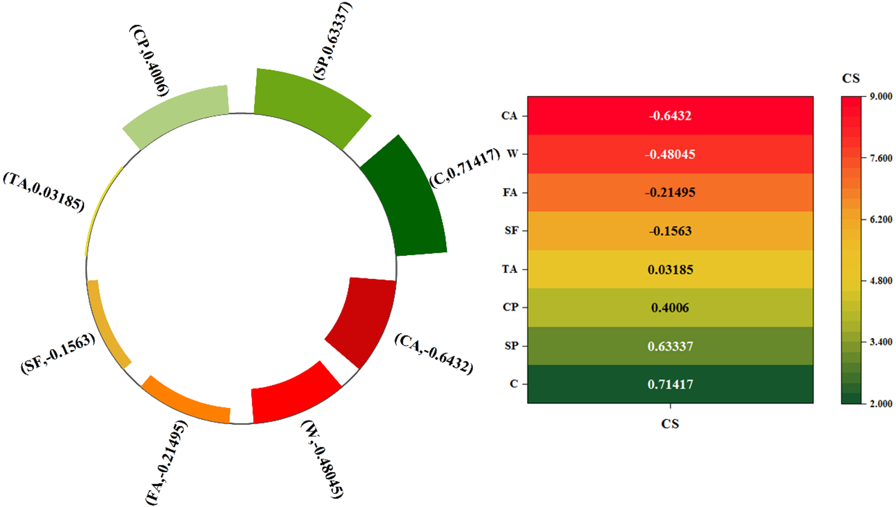
The input heat map of admixtures rate of impacts on compressive strength.

Fig. 2

The histogram of input and output variables.

Fig. 3

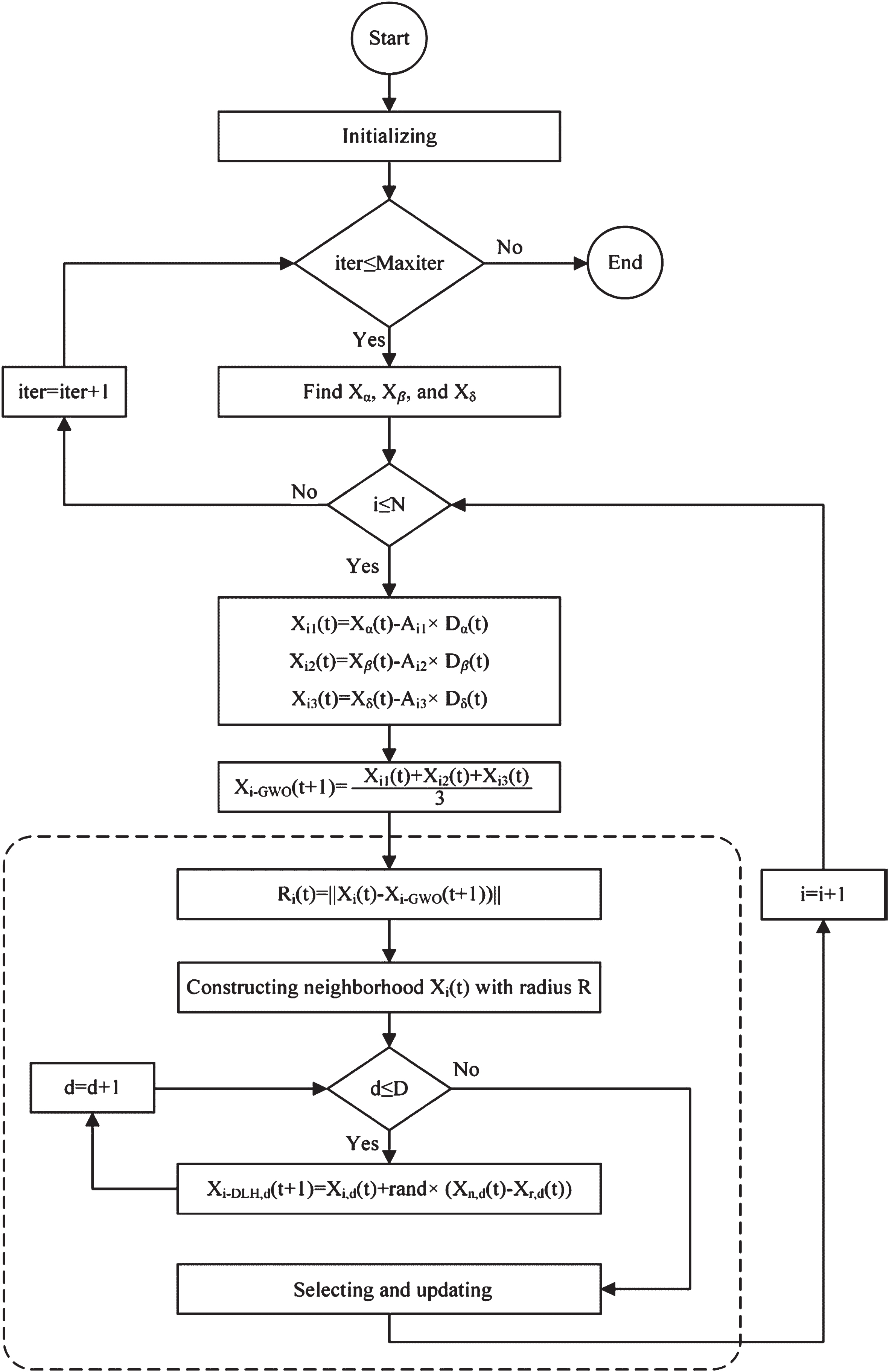
The flow chart of the I-GWO algorithm [35].

2.2 Improved Grey Wolf optimizer (I_GWO)

In Grey Wolf optimizer, αβ, δ, and ω wolf lead to areas of promising to explore space to find the optimal answer. The locally optimal solution may contain this demeanor. The cause of GWO falling within the local optimal range is reduced population variety. This section proposes an improved Gray Wolf Optimizer (I_GWO) to solve these problems. Improvements contain new explore strategies related to the update and selection procedures outlined in the dashed box in the I_GWO Fig. 4’s flowchart. Next, I_GWO contains three steps: initialization, motion, selection, and update.

Fig. 4

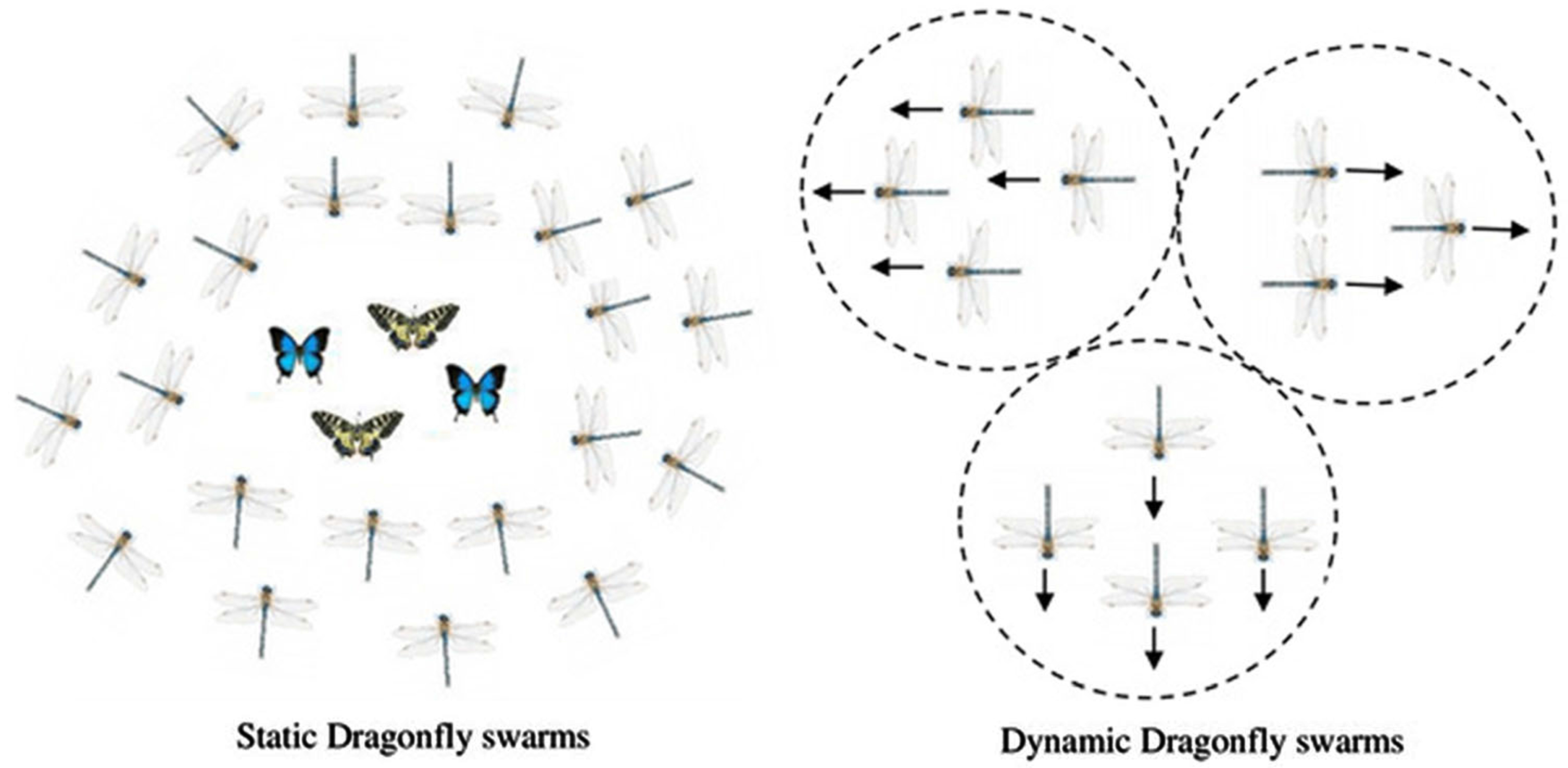
The dynamic and static swarming dragonflies’ demeanor [36].

Initialization step: In this step, n wolves are randomly placed in the explore space of a specific area [t_j, v_j] according to Equation (1)

$\begin{matrix} Y_{ij} = t_{j} + r_{j} [0, 1] \times (v_{j} - t_{j}) i \\ = [1, n], j = [1, d] \end{matrix}$ (1)

The ith wolf’s location in the tth iteration is defined as a real number of vector Y_i (t) = { y_i1, y_i2, . . . , y_id } , that d is the dimension number in the issue. The entire wolf population is stored in the n-by-d matrix Pop. By the fitness function f (Y_i (t)), The Y_i (t) the fitness value is computed. Motion Step: Moreover, to group hunting, lonely hunting is another interesting aspect of social grey wolves’ demeanor that is the motivation for improving GWO. I_GWO includes an additional mobility method called the Dimension Learning-Based Hunting (DLH) search method. At DLH, each wolf learns from its neighbors to be another candidate for a new location in Y_i (t). How a legitimate GWO and DLH explore strategy can generate two different candidates in the following steps. Regular GWO explores method: GWO considers the top three wolves in pop to be α, β, and δ.

Then the linearly reduced coefficients a and the coefficients e and F are given by Equations (2–4). The siege of the prey is then specified by determining the Y_α, Y_β, and Y_δ positions by equations (5 and 6). In general, Y_i-GWO (t + 1) is the first candidate for a new position in wolf Y_i (t) and given in equation (7):

$B = 2 {Bp}_{1} - e (t)$ (2)

$F = 2 p_{2}$ (3)

$e (t) = 2 - (2 \times t) / Maxiter$ (4)

${\begin{matrix} {\vec{B}}_{Alpha} = | {\vec{F}}_{1} \times {\vec{Y}}_{Alpha} (t) - \vec{Y} | \\ {\vec{B}}_{Beta} = | {\vec{F}}_{2} \times {\vec{Y}}_{Beta} (t) - \vec{Y} | \\ {\vec{B}}_{Delta} = | {\vec{F}}_{3} \times {\vec{Y}}_{Delta} (t) - \vec{Y} | \end{matrix}$ (5)

${\begin{matrix} {\vec{Y}}_{1} = {\vec{Y}}_{Alpha} - {\vec{Y}}_{1} \times {\vec{B}}_{Alpha} \\ {\vec{Y}}_{2} = {\vec{Y}}_{Beta} - {\vec{Y}}_{2} \times {\vec{B}}_{Beta} \\ {\vec{Y}}_{3} = {\vec{Y}}_{Delta} - {\vec{Y}}_{3} \times {\vec{B}}_{Delta} \end{matrix}$ (6)

$\vec{Y} (t + 1) = \frac{{\vec{Y}}_{1} + {\vec{Y}}_{2} + {\vec{Y}}_{3}}{3}$ (7)

p₁, p₂: random vectors in the range [0,1].

e: the vector’s elements are linearly decreased from 2 to 0.

Dimensional Learning-Based Hunting (DLH) Explore method: The original GWO creates a new location for each wolf with the three pop leader wolves’ help. Thus, GWO converges slowly, population diversity is lost too quickly, and wolves are trapped at the local optimum. The proposed DLH foraging strategy considers the individual wolves’ hunting learned to address these deficiencies from their neighbors.

The new location in each dimension of the wolf Y_i (t) is given by Equation (8) in the DLH explore method. This single wolf learns from a randomly chosen wolf learns from pop and its various neighbors. Next, in addition to Y_i-GWO (t + 1) the DLH explore method will generate another candidate for a new location in the wolf Y_i (t) named Y_i-DLH (t + 1). For this purpose, the radius P_i (t) is first computed according to equation (9) utilizing the Euclidean space between the Y_i (t)’s current location and the candidate’s location Y_i-GWO (t + 1):

$P_{i} (t) = Y_{i} (t) - Y_{i - GWO} (t + 1)$ (8)

Next, the neighborhood of Y_i (t) represented by M_i (t) is given by Equation (10). It is related to the radius P_i (t), where B_i is the Euclidean distance between Y_i (t) and Y_j (t):

$\begin{matrix} M_{i} (t) \\ = {Y_{j} (t) | B_{i} (Y_{i} (t), Y_{j} (t)) ⩽ P_{i} (t), Y_{j} (t) \in Pop} \end{matrix}$ (9)

When the Y_i (t)’s neighborhood is produced, the multi-neighborhood learning is given by Equation (11). Here, the d-dimension of Y_i-DLH (t + 1) is the d-dimension of the random neighbors Y_N,D (t) selected from M_i (t) and the random wolf Y_N,D (t) is computed by used in pop:

$\begin{matrix} Y_{i - DLH, D} (t + 1) \\ = Y_{i, D} (t) + r (M_{N, D} (t) - M_{N, D} (t)) \end{matrix}$ (10)

Selection and update step: In this step, the better candidate is first selected by comparing the goodness of fit values of the two candidates Y_i-GWO (t + 1) and Y_i-DLH (t + 1) according to equation (12), increase:

$\begin{matrix} Y_{i} (t + 1) \\ = {\begin{matrix} Y_{i - GWO} (t + 1), iff (Y_{i - GWO}) < f (Y_{i - DLH}) \\ Y_{i - DLH} (t + 1) otherwise \end{matrix} \end{matrix}$ (11)

After that, to update the Y_i (t + 1)’s the new location, if the selected candidate’s fitness value is lower than Y_i (t), then Y_i (t) is updated by the selected candidate. Y_i (t) is pop and unchanged. In general, after this process has been run for all individuals, the repetition counter (Iter) is incremented by one, and the exploration can be repeated until the predefined number of repetitions (MaxIter) is reached.

2.3 Dragonfly optimization algorithms (DA)

Developed by Mirjalili in 2016, Dragonfly Algorithm (DA) is a new, interesting, and naturally inspired metaheuristic optimization algorithm e to solve optimization’s various issues [34]. A dragonfly is a small flying carnivorous insect that hunts and eats a small insect variety such as bees, butterflies, mosquitoes, and ants. There are 3000 dragonfly types, and their life cycle has two phases: nymphs and adults. DA is according to the natural static (eating) and dynamic (moving) swarm dragonfly’s demeanor. Static and dynamic herds are shown in Fig. 5. Form a DA exploration or utilization stage. At the prey stage, the dragonfly moves the flock over long spaces in one direction, distracting the enemy. Nevertheless, during the exploration stage, dragonflies form small groups and move back and forth between small areas to attract flying prey in search of food.

Fig. 5

The dynamic and static swarming dragonflies’ demeanor [36].

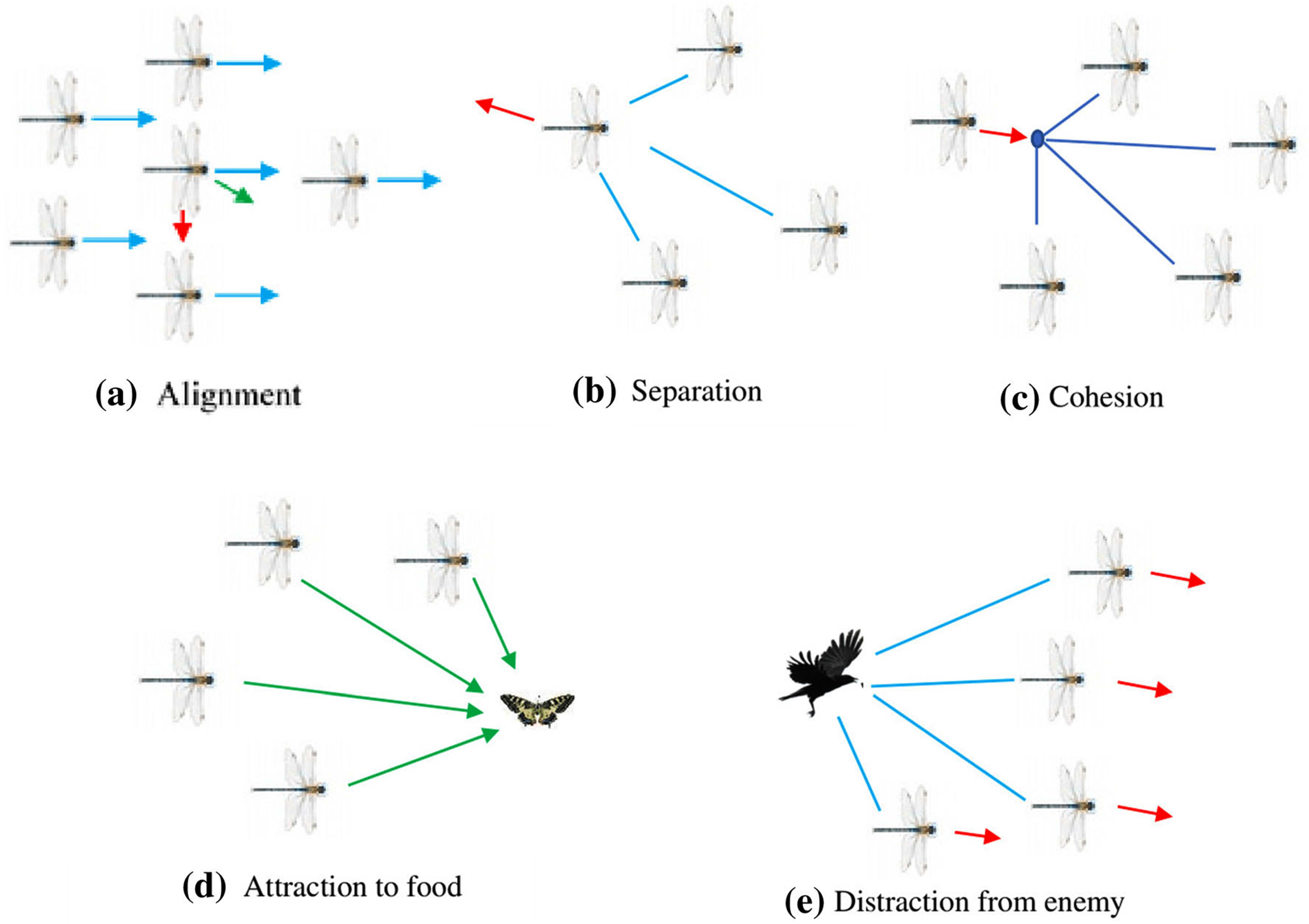
Using the five basic principles shown in Fig. 6, model the dragonfly swarm demeanor as follows: The Equation follows, Y represents the current position of the individual, Y_j Indicates the location of the jth adjacent individual, and n represents the adjacent individuals’ number.

Separation represents static collision avoidance that an individual follows to avoid collisions with another individual in the neighborhood. It is modeled mathematically by equation (12).

The alignment shows an individual’s speed match among adjacent individuals in the same group. The alignment is expressed by equation (13). Where W_i indicates the velocity of the ith individual.

Cohesion shows an individual’s tendency towards a group of herds’ centers. This is described in equation (14).

The attraction to food sources (A) is mathematically modeled by equation (15). Where A_i represents the food source for the ith individual and Y⁺ is the location of the food source.

Deflection from the enemy is mathematically modeled by equation (16). Here, D_i indicates the location of the ith individual’s enemy, and Y^- indicates the position of the enemy.

$F_{i} = - \sum_{i = 1}^{n} Y - Y_{i}$ (12)

$E_{i} = \frac{\sum_{i = 1}^{n} W_{i}}{n}$ (13)

$S_{i} = \frac{\sum_{i = 1}^{n} Y_{i}}{n} - Y$ (14)

$A_{i} = Y^{+} - Y$ (15)

$D_{i} = Y^{-} - Y$ (16)

Fig. 6

RBF neural network [37].

The position of the artificial register mark in the search space is updated, taking into account the vector’s step ΔY and the Y position vector. The ΔY step vector is similar to the velocity vector of the PSO algorithm. It is stated and updated in the following:

$\begin{matrix} Δ Y (y + 1) \\ = ({fF}_{i} + {eE}_{i} + {sS}_{i} + {aA}_{i} + {dD}_{i}) + g Δ Y_{n} \end{matrix}$ (17)

Here, f defines the split point, F_i defines the split point of the i^th instance, e, E_i defines the i^th association and split points, respectively. s, S_i determine the association score and the association score of the i^th instance, respectively. a, A_i determine the food agent and food source of individual i^th, respectively. d, D_i determine the agent of the enemy and the location of the enemy of the i^th instance, respectively. g, as in the PSO algorithm, defines the inertial weight. n defines the number of iterations.

Next, the ith dragonfly’s location at t + 1 is updated in the following:

$Y_{t + 1} = Y_{t} + Δ Y_{t + 1}$ (18)

Exploration is ensured by employing high association and low coherence weight. Nevertheless, mining is guaranteed by employing low linking and high consolidation weights. The rate of convergence of the DA can be controlled by adaptively adjusting the weights (f), (e), (s), (a), and (d). To improve the search, randomization, and artificial dragonflies’ exploitation, a random walk (Levy flight) is introduced in the absence of an adjacent solution. Therefore, the position of the i^th dragonfly at repetition t + 1 is updated in the following:

$Y_{t + 1} = Y_{t} + Levy (D) \times Y_{t}$ (19)

Where D represents the dimensionality of the position vector, the sample flights are computed from:

$Levy (D) = 0.01 \times \frac{p_{1} \times δ}{{| p_{2} |}^{\frac{1}{α}}}$ (20)

p₁andp₂ define random numbers in the range [1,0]. α defines a constant value.

δ is given by equation 21 below:

$δ = {(\frac{μ (1 - α) \times sin (\frac{π α}{2})}{μ (\frac{1 - α}{2}) \times α \times 2^{(\frac{α - 1}{2})}})}^{\frac{1}{α}}$ (21)

Here, μ (x) = (x - 1)

2.4 Radial basis function (RBF)

Radial basis function neural network (RBFNN) is employed in several control methods, including predictive model control and sliding mode control. It is known as a useful strategy to solve control problems in the indeterminate model system. To overcome the previous passivity problem in traditional teleoperation systems with the energy signals’ transmission, a unique communication mode has been developed in the communication channel to transmit estimated environmental parameters without energy. Accordingly, RBF neural networks aim to address master modeling uncertainty and parameter variability, model environmental dynamics through slave manipulator dynamics, and estimate ecological parameters by discussing performance improvements for different neural networks and experimenting with other neural network types, and future research may be possible.

The first definition is the feedforward radial basis function neural network is designed to include three layers: n inputs, n hidden nodes, and 1 output, as shown in Fig. 7. The variables are just weights from the hidden layer to the output layer.

Fig. 7

The scatter presentation of the correlation between measured and predicted values of compressive strength.

Describe input u = [u₁ … u₂ … u_n] ^P and can get the Gaussian function as follows:

$K_{i} (U) = exp (- \frac{u - {vi}^{2}}{2 L_{i}^{2}}) i = 1, 2 \dots, n$ (22)

L_i indicate the Known parameters of the Gaussian function, v_i = [v_i1 … v_ij … v_in] ^P

u - vi²: Shows the Euclidean Norm, K_i = [K₁ … K_i … K_n] ^P

To describe the vi’s choice:

I = [v₁ … v_j … v_n] ^P: indicates to include different v_i indifferent layers.

Next, the output of the RBF neural network is the linear weighted the n’s sum basis functions derived in the following:

$F_{l} = \sum_{i = 1}^{n} t_{il} K_{i} (U)$ (23)

t_i: the weights of output.

F_l: the output value.

2.5 Evaluation criteria

Table 2 calculates various indicators to evaluate the model’s performance that produces compressive strength (CS) values for HPC samples during the calibration and validation phases. The indicator contains the coefficient of determination (R²): $R^{2} = {(\frac{\sum_{i = 1}^{n} (p_{i} - \bar{p}) (t_{i} - \bar{t})}{\sqrt{[\sum_{i = 1}^{n} {(p_{i} - \bar{t})}^{2}] [\sum_{i = 1}^{n} {(t_{i} - \bar{t})}^{2}]}})}^{2}$

Root means square error (RMSE): $RMSE = \sqrt{\frac{1}{n} \sum_{i = 1}^{n} {(t_{i} - p_{i})}^{2}}$

Scatter index (SI): $SI = \frac{RMSE}{mean (x_{i})}$

RMSE-observations standard deviation ratio (RSR): $RSR = \frac{RMSE}{St . Dev}$

Coefficient of persistence (CP): $cp = 1 - \frac{\sum_{i = 2}^{n} {(p_{i} - t_{i})}^{2}}{\sum_{i = 1}^{n - 1} {(p_{i + 1} - t_{i})}^{2}}$

n10_index: $n 10 - index = \frac{n 10}{n}$

Here, p_i shows the ith estimated CS employing models, t_i indicates the ith observed CS. In addition, n indicates the sample number, $\bar{t}$ and $\bar{p}$ show the mean value of estimated and predicted, respectively

3 Results and discussion

Predicting the compressive strength of high-performance concrete needs advanced models, algorithms, and enhancements. As already mentioned, the RBF model and the two algorithms I_GWO and DA, are used as the optimizer for this model. Furthermore, the response and output of the 2 combined models, I_GWO_RBF and DA_RBF, are compared to choose the simple model and algorithm. There are 3 levels of this model: input, hide, and output. This estimate and model use parameters that indicate each modeling error and the min and max size. As already mentioned, the two models are a combination of two parts, learning and validation, and are compared utilizing the figures and shapes of two parts and two models. The learning part accounts for 70% of the sample, and the validation part makes up 30% of the sample. Therefore, the error rate in the field of education will be much higher than in the field of testing. Nevertheless, it is important to note which hidden layer algorithm performed better optimizations on the RBF model and achieved satisfactory performance and output.

To compare the present work fairly with the literature, some papers that utilized the same dataset in their implementation were chosen. The R² and RMSE values are selected to enlighten the robustness of the present work. According to the evaluator parameters, the present work shows better values.

Table 3 shows the modeling done according to evaluators. The estimators include R², RMSE, SI, RSR, CP, and n10_index. For the R² parameter, which is the highest value indicating the best state, the IGWO_RBF model has the highest value of 96.99% in the validation section. On the other hand, DA_RBF in the learning section had the lowest value, equal to 95.69. In this parameter, both models have performed closely in both sections and have obtained acceptable values.

In terms of RMSE, SI, RSR, and CP parameters, unlike R², the lowest value represents the best state. In RMSE and SI, the lowest values are 2.9575 and 0.0459, respectively, belonging to IGWO_RBF in the learning section. Also, the highest value of these two parameters belongs to DA_RBF in the learning section, with a value equal to 3.0364 for the RMSE parameter and SI with a value equal to 0.0478 in the validation section. RSR in the validation section related to the IGWO_RBF model is equal to 0.1751, which is the most suitable value, and the weakest performance related to the DA_RBF model in the learning section is equal to 0.2072. However, on the other hand, for the CP of the DA_RBF model in the learning section, the best value is equal to 142.73, and also the worst case for this model, but in the validation section. In the n10_index parameter, like the R² parameter, the highest value indicates that the best mode belongs to the learning section in the DA_RBF model, and the weakest performance is related to the same DA_RBF model in the validation section. In general, according to Table 2, it is clear that the combined IGWO_RBF model has been able to show better performance.

Table 2
Comparison of present work with similar research in the literature

Work title Model Compressive strength

R2 RMSE

Huang et al. [38] Mars-PSBBO 0.942 4.3169

Yin et al. [39] Mars 0.962 3.3909

Present work IGWO_RBF 0.9699 2.9779

Work title	Model	Compressive strength
Huang et al. [38]	Mars-PSBBO	0.942	4.3169
Yin et al. [39]	Mars	0.962	3.3909
Present work	IGWO_RBF	0.9699	2.9779

Table 3

Developed models’ assessment results by evaluators

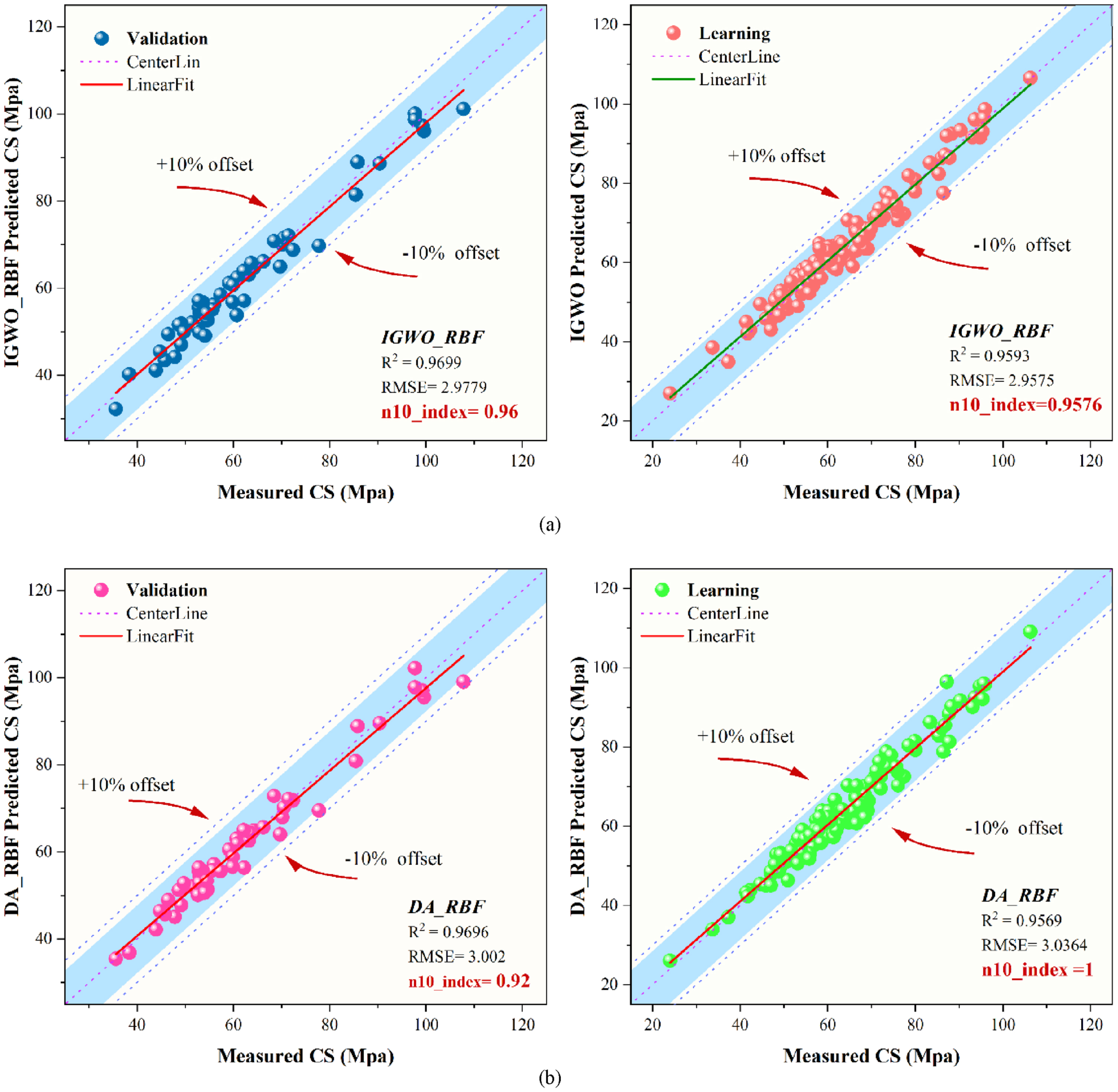
Figure 8 indicates the scatter presentation of the correlation between measured and predicted compressive strength values in the learning and validating phase. Each point in this figure shows the measured and predicted samples. The center line is in the coordinate of X = Y, and if the points were close to the center line, that determined the suitable performance. Furthermore, the linear fit denotes all samples’ midpoints, and the angle difference between the linear fit and center line indicates the weak or strong performance of the respective models. In addition, there are two support lines below and above the center line. If the sample intersects the top or bottom of the related lines, the points are said to be overestimated or underestimated, respectively, according to three parameters, R², RMSE, and n10_index. A high R², n10_index, and a low RMSE illustrate low variance and high density.

Fig. 8

The error percentage diagram of developed models.

In general, R² and RMSE determine the points’ location and the points’ dispersion in the series, respectively. According to the figure shown, it can be seen that the models had almost the same performance. In the comparison of the models in the validation section, due to the fact that the values of the parameters in IGWO_RBF were more suitable than DA_RBF, as a result, less dispersion was observed in IGWO_RBF. Also, DA_RBF has been underestimated in some places. On the other hand, in the learning section, despite the fact that DA_RBF has obtained high values in R² and n10_index but has more RMSE, it has relatively high dispersion compared to IGWO_RBF.

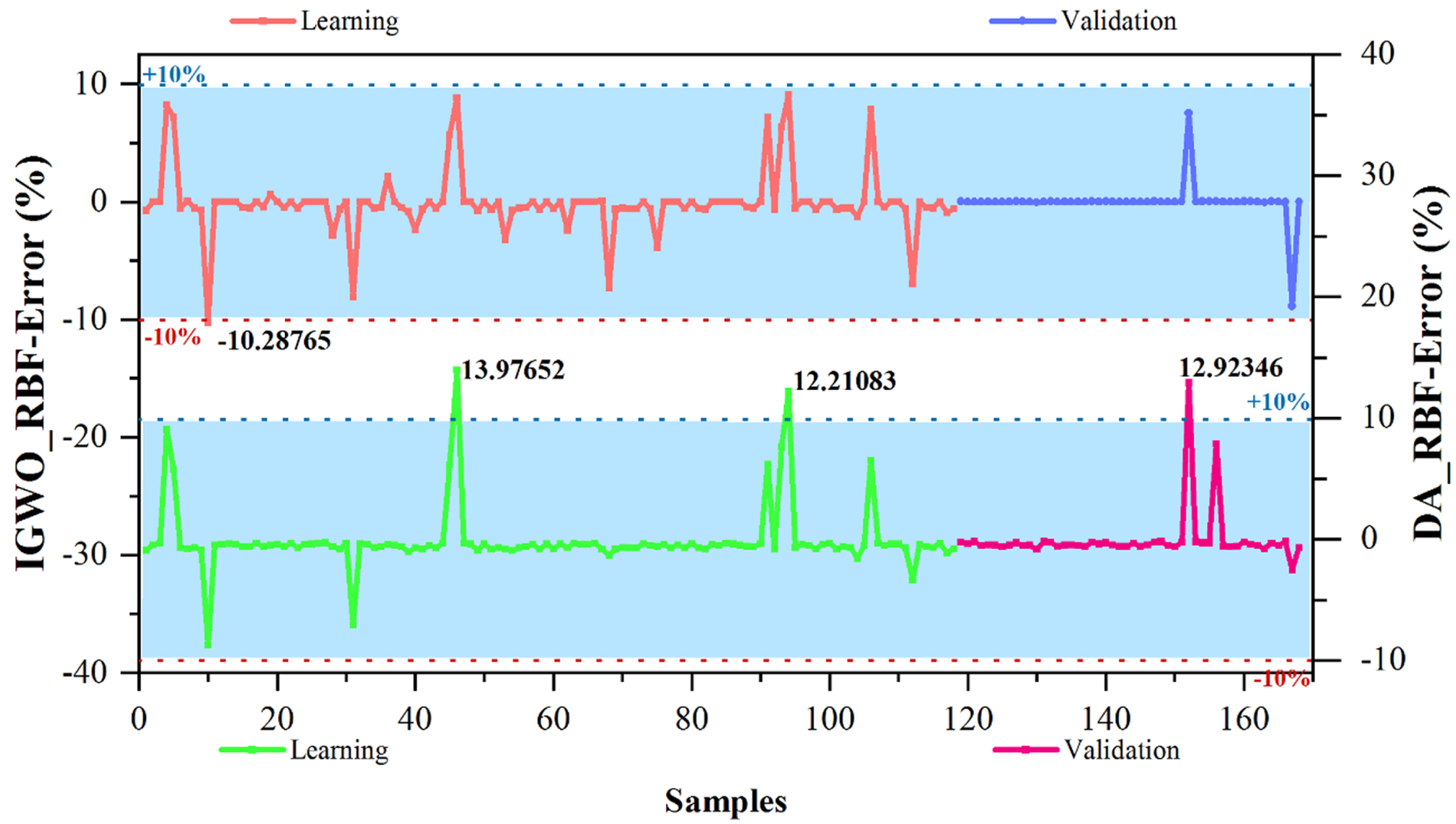
Figure 9 indicates the percent error percentage diagram of developed models. The relevant diagram has been evaluated in the learning and validation section, and as mentioned, 70% and 30% of the samples have been allocated to these sections, respectively. Fluctuations in this diagram are desirable to be between the 10 and – 10 percent range. If any fluctuation is outside these numbers, it indicates an excessive error. In the learning part DA_RBF model, the highest value obtained in this section equals 13.97%, which has improved its performance to 12.92% in the validation section. The significant point in the values obtained in the two sections is that if the performance improvement is seen in the validation section, the result was a good training of the examples in the learning section. In IGWO_RBF, the highest error percentage was equal to 10.28%, almost 3% lower than DA_RBF. In addition, IGWO_RBF has reduced its error below 10% by improving its performance and better training, which was almost 9%. In general, comparing the two models, it can be concluded that the error of IGWO_RBF in the two parts of learning and validation is more than that of DA_RBF, which is the result of the high accuracy of the model.

Fig. 9

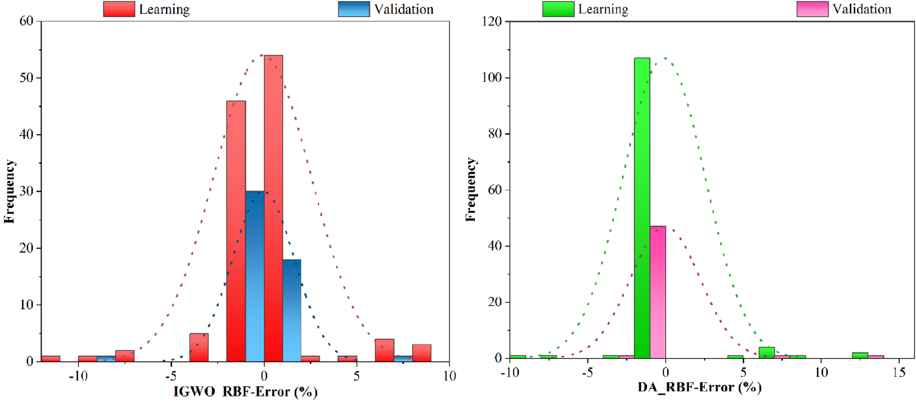
The error percentage density histogram.

Figure 10 shows the error percentage density histogram in both combined models of this article. In the specified figure for the IGWO-RBF model, the error density was in the middle and was approximately in the range of – 2.5 to 2.5. The highest error percentage, equal to 12%, involved only approximately 1 frequency in the learning section. The validation section, as well as the learning section, has a sharp normal distribution and follows the normal state, which indicates the low dispersion of errors in the two relevant sections, and the frequency of errors in the validation section was close to zero percent. On the other hand, for DA_RBF in the learning section, as it is clear in the figure, the dispersion of errors is much higher, which has caused a slight right skew. But most of the frequency of errors was in the zero interval, which obtained the normal distribution of sharpness. In the validation section related to DA_RBF, it can be seen that it performed like the learning section, so that most of the frequency of errors was in the zero percent range, but the dispersion of errors created a flatter normal distribution than IGWO_RBF. In general, it was observed that the performance of IGWO_RBF in both sections was more appropriate than DA_RBF, considering that it has more density in the zero percent range and a sharper normal distribution.

4 Conclusion

High-performance concrete (HPC) is compared to conventional concrete, which exhibits superior durability, workability, and strength performance. Its improved attributes are chemical additives and the addition of additional cement-based material. Supplemental cement-based materials like crushed blast furnace slag, silica fume, and fly ash can help reduce costs, save energy and resources, and protect the environment from impact while significantly improving concrete properties. CS is a function of 8 inputs, including water, coarse and fine aggregate, silica fume, cement, superplasticizer, fly ash, and concrete age. The model’s results are more exact than those using nonlinear regression analysis. ANN models were built at different ages to predict the fly ash HPC’s compressive strength. The model was trained on the Portland cement’s weight and utilizing sample age, fly ash, water, a highly efficient water-reducing agent, two crushed stone types, sand, and a 1 concrete cubic meter lime fraction. Artificial neural network (ANN) was developed in architecture with artificial intelligence’s expansion. The result was more accurate for predicting concrete strength than classic regression analyses. Using RBFNN to predict the fly ash concrete’s strength, it was found that the prediction method was easy, feasible, accurate, and could have a wide range of applications. The RBF model is used to predict the compressive strength of high-performance concrete. Two optimization algorithms are used to optimize this type of modeling and achieve results close to the laboratory sample. Both use innovative Improved Grey Wolf optimizer (I_GWO) and Dragonfly optimization algorithms (DA) to achieve better optimization results. These two optimizers are described in detail below. The results of the two combined models are as follows:

For the R² parameter, the IGWO_RBF model has the highest value of 96.99% in the validation section. On the other hand, DA_RBF in the learning section had the lowest value, equal to 95.69.

For RMSE, the lowest values are 2.9575, which belongs to IGWO_RBF in the learning section. Also, the highest value of this parameter belongs to DA_RBF in the learning section, with a value equal to 3.0364.

For SI, the lowest value is 0.0459, which belongs to IGWO_RBF in the learning section. Also, the highest value of this parameter belongs to DA_RBF, equal to 0.0478 in the validation section.

RSR in the validation section related to the IGWO_RBF model equals 0.1751, which is the most suitable value, and the weakest performance related to the DA_RBF model in the learning section is equal to 0.2072.

For the CP of the DA_RBF model in the learning section, the best value equals 142.73, and the worst case for this model, but in the validation section.

In the n10_index parameter, the highest value indicates the best mode belongs to the learning section in the DA_RBF model equal to 1, and the weakest performance is related to the same DA_ RBF model equal to 0.92 in the validation section.

References

Peng

C.-H.

, Yeh

I.-C.

and Lien

L.-C.

, Building strength models for high-performance concrete at different ages using genetic operation trees, nonlinear regression, and neural networks, Eng Comput 26(1) (2010), 61–73.

Khan

M.I.

, Predicting properties of high performance concrete containing composite cementitious materials using artificial neural networks, Autom Constr 22 (2012), 516–524.

Ahmadi-Nedushan

, An optimized instance based learning algorithm for estimation of compressive strength of concrete, Eng Appl Artif Intell 25(5) (2012), 1073–1081.

Aïtcin

P.-C.

, High performance concrete. CRC press, 1998.

Behnood

, Behnood

, Gharehveran

M.M.

and Alyamac

K.E.

, Prediction of the compressive strength of normal and high-performance concretes using M5P model tree algorithm, Constr Build Mater 142 (2017), 199–207.

Kim

J.-I.

, Kim

D.K.

, Feng

M.Q.

and Yazdani

, Application of neural networks for estimation of concrete strength, J Mater Civ Eng 16(3) (2004), 257–264.

Atici

, Prediction of the strength of mineral admixture concrete using multivariable regression analysis and an artificial neural network, Expert Syst Appl 38(8) (2011), 9609–9618.

Yeh

I.-C.

, Modeling of strength of high-performance concrete using artificial neural networks, Cem Concr Res 28(12) (1998), 1797–1808.

Bhanja

and Sengupta

, Investigations on the compressive strength of silica fume concrete using statistical methods, Cem Concr Res 32(9) (2002), 1391–1394.

10.

Lim

C.-H.

, Yoon

Y.-S.

and Kim

J.-H.

, Genetic algorithm in mix proportioning of high-performance concrete, Cem Concr Res 34(3) (2004), 409–420.

11.

Topcu

I.B.

and Sarıdemir

, Prediction of compressive strength of concrete containing fly ash using artificial neural networks and fuzzy logic, Comput Mater Sci 41(3) (2008), 305–311.

12.

Dias

W.P.S.

and Pooliyadda

S.P.

, Neural networks for predicting properties of concretes with admixtures, Constr Build Mater 15(7) (2001), 371–379.

13.

Hearst

M.A.

, Dumais

S.T.

, Osuna

, Platt

and Scholkopf

, Support vector machines, IEEE Intell Syst their Appl 13(4) (1998), 18–28.

14.

Chen

, Study of applying macroevolutionary genetic programming to concrete strength estimation, J Comput Civ Eng 17(4) (2003), 290–294.

15.

Yeh

I.-C.

and Lien

L.-C.

, Knowledge discovery of concrete material using genetic operation trees, Expert Syst Appl 36(3) (2009), 5807–5812.

16.

Latif

S.D.

, Concrete compressive strength prediction modeling utilizing deep learning long short-term memory algorithm for a sustainable environment, Environ Sci Pollut Res 28(23) (2021), 30294–30302.

17.

Chen

and Li

, Using The Support Vector Regression Model With IGWO And DA Algorithms To Predict High-performance Concrete’s Compressive Strength, J Appl Sci Eng 26(8) (2022), 1175–1187.

18.

Kandiri

, Sartipi

and Kioumarsi

, Predicting Compressive Strength of Concrete Containing Recycled Aggregate Using Modified ANN with Different Optimization Algorithms, Appl Sci 11(2) (2021), 485. doi: 10.3390/app11020485.

19.

Prasad

B.K.R.

, Eskandari

and Reddy

B.V.V.

, Prediction of compressive strength of SCC and HPC with high volume fly ash using ANN, Constr Build Mater 23(1) (2009), 117–128.

20.

Pedro

and de

, Brito and L. Evangelista, Durability performance of high-performance concrete made with recycled aggregates, fly ash and densified silica fume, Cem Concr Compos 93 (2018), 63–74. doi: 10.1016/j.cemconcomp.2018.07.002.

21.

Hammoudi

, Moussaceb

, Belebchouche

and Dahmoune

, Comparison of artificial neural network (ANN) and response surface methodology (RSM) prediction in compressive strength of recycled concrete aggregates, Constr Build Mater 209 (2019), 425–436.

22.

Chou

J.-S.

and Pham

A.-D.

, Enhanced artificial intelligence for ensemble approach to predicting high performance concrete compressive strength, Constr Build Mater 49 (2013), 554–563.

23.

H.-G.

and Wang

J.-Z.

, Prediction of compressive strength of concrete by neural networks, Cem Concr Res 30(8) (2000), 1245–1250.

24.

Saberi-Movahed

, Najafzadeh

and Mehrpooya

, Receiving more accurate predictions for longitudinal dispersion coefficients in water pipelines: training group method of data handling using extreme learning machine conceptions, Water Resour Manag 34(2) (2020), 529–561.

25.

Najafzadeh

and Tafarojnoruz

, Evaluation of neuro-fuzzy GMDH-based particle swarm optimization to predict longitudinal dispersion coefficient in rivers, Environ Earth Sci 75(2) (2016), 157. doi: 10.1007/s12665-015-4877-6.

26.

Ren

and Zhao

, An optimal neural network and concrete strength modeling, Adv Eng Softw 33(3) (2002), 117–130.

27.

Panda

and Narasimhan

, Forecasting daily foreign exchange rate in India with artificial neural network, Singapore Econ Rev 48(02) (2003), 181–199.

28.

Supharatid

, Tidal-level forecasting and filtering by neural network model, Coast Eng J 45(01) (2003), 119–137.

29.

Masoumi

, Najjar-Ghabel

, Safarzadeh

and Sadaghat

, Automatic calibration of the groundwater simulation model with high parameter dimensionality using sequential uncertainty fitting approach, Water Supply 20(8) (2020), 3487–3501. doi: 10.2166/ws.2020.241.

30.

Kramer

M.A.

, Nonlinear principal component analysis using autoassociative neural networks, AIChE J 37(2) (1991), 233–243.

31.

Dong

and McAvoy

T.J.

, Nonlinear principal component analysis— based on principal curves and neural networks, Comput Chem Eng 20(1) (1996), 65–78.

32.

Yamazaki

and Ludermir

T.B.

, Neural network training with global optimization techniques, Int J Neural Syst 13(02) (2003), 77–86.

33.

Lam

, Wong

Y.L.

and Poon

C.-S.

, Effect of fly ash and silica fume on compressive and fracture behaviors of concrete, Cem Concr Res 28(2) (1998), 271–283.

34.

Mirjalili

, Dragonfly algorithm: a new meta-heuristic optimization technique for solving single-objective, discrete, and multi-objective problems, Neural Comput Appl 27(4) (2016), 1053–1073.

35.

Nadimi-Shahraki

M.H.

, Taghian

and Mirjalili

, An improved grey wolf optimizer for solving engineering problems, Expert Syst Appl 166 113917, 2021.

36.

Meraihi

, Ramdane-Cherif

, Acheli

and Mahseur

, Dragonfly algorithm: a comprehensive review and applications, Neural Comput Appl 32(21) (2020), 16625–16646.

37.

Chen

, Huang

, Sun

, Gu

and Yao

, RBF-neural-network-based adaptive robust control for nonlinear bilateral teleoperation manipulators with uncertainty and time delay, IEEE/ASME Trans Mechatronics 25(2) (2019), 906–918.

38.

Huang

, Jiang

, Wang

, Zhu

and Afzal

, Prediction of long-term compressive strength of concrete with admixtures using hybrid swarm-based algorithms, Smart Struct Syst 29(3) (2022), 433–444.

39.

Yin

, Liu

, Lu

, Nie

and Jia

, Prediction of the compressive and tensile strength of HPC concrete with fly ash and micro-silica using hybrid algorithms, Adv Concr Constr 12(4) (2021), 339–354.

Variables	Statistical properties
Max	Min	Ave	St.dev
Fly ash (kg/m³)	275	0	101.07	66
Silica fume (kg/m³)	43	0	21.8	17.9
Superplasticizer (kg/m³)	13	0	4.47	3.1
Coarse aggregates (kg/m³)	1157	1086	1133.6	24.4
Total aggregates (kg/m³)	1867	1668	1805.7	63.2
Water (kg/m³)	205	118.2	165.6	28.7
Cement (kg/m³)	500	400	418.4	40.1
Curing days (day)	180	28	68	50
Compressive strength (MPa)	107	24	64	15.3

Predicting the compressive strength of High-performance concrete by using Radial basis function with optimization Improved Grey Wolf optimizer and Dragonfly algorithm

Abstract

Keywords

1 Introduction

2 Materials and methodology

2.1 Data gathering

3 Results and discussion

Table 2 Comparison of present work with similar research in the literature Work title Model Compressive strength R2 RMSE Huang et al. [38] Mars-PSBBO 0.942 4.3169 Yin et al. [39] Mars 0.962 3.3909 Present work IGWO_RBF 0.9699 2.9779

References

Table 2
Comparison of present work with similar research in the literature

Work title Model Compressive strength

R2 RMSE

Huang et al. [38] Mars-PSBBO 0.942 4.3169

Yin et al. [39] Mars 0.962 3.3909

Present work IGWO_RBF 0.9699 2.9779