
Abstract
In this paper, bipolar fuzzy planar graph is defined and studied several properties. The bipolar fuzzy planar graph is defined in a very interesting way. The parameter “degree of planarity” measures the planarity of a bipolar fuzzy graph. The other relevant terms such as strong edges, bipolar fuzzy faces, strong bipolar fuzzy faces are defined here. A very close association of bipolar fuzzy planar graph is bipolar fuzzy dual graph. This is also defined and several properties of it are studied. Bipolar fuzzy planar graph and bipolar fuzzy dual graph have many applications in different fields including design of social network, design of subway tunnel or routes, gas or oil pipelines, image segmentation, etc.
Keywords
Introduction
Graph theory is now become an important topic in research area due to its application in real world. There are many real world applications of graph theory in which crossing between edges is complicated such as computer networks, circuit designing, subways, utility lines, flyovers, etc. After the development of graph theory, Rosenfeld [26] introduced fuzzy graph theory and then, the fuzzy graph theory is growing rapidly with a large number of branches. In 1998, the concept of bipolar fuzzy set is introduced by Zhang [39] as a generalization of fuzzy set. A bipolar fuzzy set is a generalization of Zadeh’s fuzzy set. Authors may refer [2, 28–30] for more information on fuzzy sets as well as on fuzzy graphs. Abdul-jabbar et al. [1] and Nirmala and Dhanabal [20] introduced the concept of fuzzy planar graph. Recently, Samanta and Pal [21, 34] introduced fuzzy planar graph in a different way. In these papers, they also introduced fuzzy faces, strong fuzzy planar graphs, fuzzy dual graphs, etc. Pramanik et al. [22] have defined interval-valued fuzzy planar graph and investigated several properties. Also, they have introduced fuzzy φ-tolerance competition graph in [23] and interval-valued fuzzy φ-tolerance competition graph in [24]. Ghorai and Pal [10, 11] have recently worked on m-polar fuzzy planar graphs. They have also discussed certain types of product bipolar fuzzy graphs in [12]. Ghorai et al. [13] have given new concepts of regularity in product m-polar fuzzy graphs. Recently, Sahoo and Pal [27] have discussed on product of intuitionistic fuzzy graphs and degree.
Due to lack of space and huge population, the necessity of flyovers, subway tunnels, metro-lines increases. But crossing of routes can be accepted, since the crossing of subway tunnels, metro-lines, etc. are very expensive in some cases. It is clear that, crossing of one congested and a low congested route is more safer than crossing of two congested route. The term “congested”, “low congested” are vague and hence can not be handled in crisp graph. These vague terms can be dealt better in bipolar fuzzy graph by assigning some positive membership and negative membership values. In general, one can try to place the communication lines at different heights when there is need to cross the lines. In case of electrical wires it is not a big issue, but it causes huge expenses for some type of lines such as, building one flyover over another. Using planar graphs, these type of problems can be modeled and inspected further for reducing the cost and space of construction. In crisp planar graphs, crossing of lines are strictly not allowed. So, in such type of modeling the real applications where crossing of lines are necessary, can not be represented by crisp planar graphs. Using decomposition of planar graphs, various computational challenges including image segmentation or shape matching is solved.athematical sense, strong route means highly congested route and weak route means low congested route. Thus in city planning, crossing between a strong route and a weak route is more safer than crossing between two strong routes.
In this modern age, image analysing, image segmenting, image shrinking, etc. are growing and useful research topic. Images are captured and stored in terms of pixel with some parametric informations such as intensity of colours, distance of pixels, size of pixels, etc. Taking pixels as vertices and intensity and non-intensity of pixels as positive and negative membership values respectively, an image information can be represented as a bipolar fuzzy graph.
Motivated from these ideas, bipolar fuzzy planar graph is introduced, which is itself a bipolar fuzzy graph with some degree of planarity. Two procedural applications namely “image shrinking” and “city planning” are discussed in Section 5.
Recently, the bipolar fuzzy graphs have been discussed in [2, 9]. In these articles, the concepts of neighbourly irregular bipolar fuzzy graphs, neighbourly totally irregular bipolar fuzzy graphs, highly irregular bipolar fuzzy graphs and highly totally irregular bipolar fuzzy graphs have been introduced. Samanta and Pal [32] have also worked on bipolar fuzzy hypergraphs. There are so many related works found in [31, 35–37].
In this paper, we defined bipolar fuzzy planar graph and bipolar fuzzy dual graph and presented several properties.
Preliminaries
A graph G = (V, E) is a representation of a set V of objects (vertices) where some pairs of objects are connected by links (edges), where the set E of such pairs is defined to be a subset of V × V. G is finite when V and E are finites. An infinite graph is one with an infinite set of vertices or edges or both. Most commonly in graph theory, it is implied that the graphs discussed are finite. A multigraph is a graph containing multiple edges and without self loops. There is no unique geometric representation of a graph.
Embedding is a geometrical representation of a graph in any surface so that no edges intersect. A graph G is planar if it can be embedded in the plane. So the graph is non-planar if it is not planar that is, it can not be drawn without crossing. A planar graph splits the plane into a set of regions, called faces. The length of a face in a planar graph G is the total length of the closed walk in G bounding the face. The portion of the plane lying outside is infinite region.
In graph theory, the dual graph of a given planar graph G is a graph which has a vertex corresponding to each faces of G, and the graph has an edge joining two neighboring faces for each edge in G, for a certain embedding of G.
A fuzzy set A on an universal set X is meant by a mapping m : X → [0, 1], which is called the membership function. A fuzzy set is denoted by A = (X, m).
A fuzzy graph [26] ξ = (V, σ, μ) is a non-empty set V with the pair of functions σ : V → [0, 1] and μ : V × V → [0, 1] such that for all x, y ∈ V, μ (x, y) ≤ min {σ (x) , σ (y)}, where σ (x) and μ (x, y) represent the membership values of the vertex x and of the edge (x, y) in ξ respectively. A loop at a vertex x ∈ V in ξ is represented by μ (x, x) ≠0. An edge is non-trivial if μ (x, y) ≠0. A fuzzy graph ξ = (V, σ, μ) is complete if μ (u, v) = min {σ (u) , σ (v)} for all u, v ∈ V, where (u, v) denotes the edge between the vertices u and v.
Several definitions of strong edge are available in literature. Among them the definition of [7] is more suitable for our purpose. The definition is given below:
For the fuzzy graph ξ = (V, σ, μ), an edge (x, y) is called strong [7] if
Let V be not an empty set. A bipolar fuzzy set (BFS) [14, 39] B in V is characterized by
For the sake of simplicity, we shall use the symbol
Let V be a nonempty set. Then we call the mapping
A bipolar fuzzy graph [2] (BFG) ξ of a (crisp) graph G = (V, E) is a pair ξ = (A, B, V, E) where
The underlying crisp graph of a BFG ξ = (A, B, V, E) is the crisp graph G = (V, E) where
A BFG ξ = (V, E, A, B) is said to be complete if
A BFG is called strong BFG if
If the vertex set V of a BFG (V, E, A, B) can be partitioned into two non-empty subsets V1 and V2 such that
Now, we define bipolar fuzzy multi-set. A multiset over a non-empty set V is simply a function d : V → N, where N is the set of natural numbers. Yager [38] first discussed fuzzy multisets, although he used the term “fuzzy bag”. An element of a non-empty set V may come more than once with the same or different membership values. A natural generalization of this elucidation of multiset heads to the notion of fuzzy multiset, or fuzzy bag, over a non-empty set V as a mapping
Bipolar fuzzy multigraph
In this section, bipolar fuzzy multigraph (BFMG) is introduced. Let V be a non-empty set. Also, let
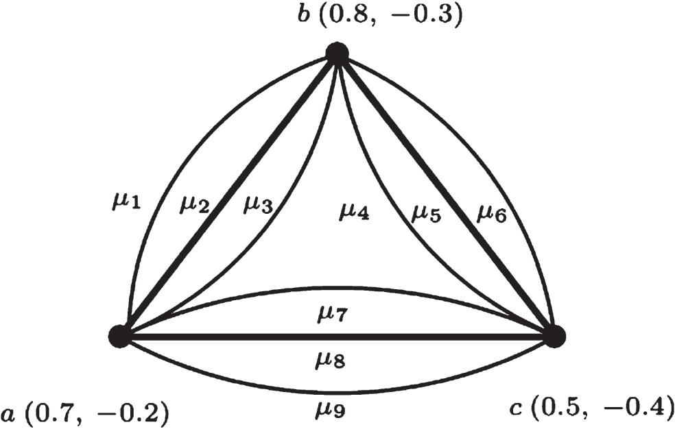
An example of bipolar fuzzy multigraph.
Planarity is foremost problem in connecting the water lines, wire lines, printed circuit design, gas lines, etc. But, some times little crossing may be accepted to these design of such lines or circuits. So bipolar fuzzy planar graph (BFPG) is an important topic for these connections.
If there is atleast one intersection of edges in all possible geometrical representation of a crisp graph, the graph is called non-planar graph. Let a crisp graph G has an intersection between two edges (a, b) and (c, d) for a certain geometrical representation. In fuzzy concept, we say that these two edges have membership value 1. If we remove the edge (c, d), the graph becomes planar. In fuzzy sense, the membership values of the edges (a, b) and (c, d) are 1 and 0 respectively.
Let ξ = (A, B, V, E) be a BFG and the graph has only one crossing between two edges
Before going to the main definition, some co-related terms are discussed below.
Intersecting value in bipolar fuzzy multigraph
The positive-strength of an edge (a, b) is measured by
Based on the values of
p-strong if n-strong if very p-strong if very n-strong if
In BFMG, when two edges intersect at a point, the value associated to that point is calculated in the following way. Let a BFMG contains two edges ((a, b),
We define the intersecting value at the point T by
It is easy to verify that the range of f is 0 < f ≤ 1.
In a certain geometrical representation of a BFPG, if there is no point of intersection then the degree of planarity of the BFPG is 1. In this case, the underlying graph of this BFPG is the crisp planar graph. If f decreases, then the number of point of intersections between the edges increases and obviously the nature of planarity decreases. From this analogy, one can say that every BFG is a BFPG graph with some degree of planarity.
The degree of planarity for the bipolar fuzzy complete graph is calculated from the following theorem.
Depending on the degree of planarity, the number of point of intersections of a BFPG can be found. The following theorem proves that there is no point of intersection between very p-strong edges if the degree of planarity is greater than 0.4.
From Theorem 2, one can identify a special kind of BFPG whose degree of planarity is more than 0.4. This type of BFPG is defined below.
From Theorem 3, one can identify a special kind of BFPG whose degree of planarity is less than 0.67. This type of BFPG is defined below.
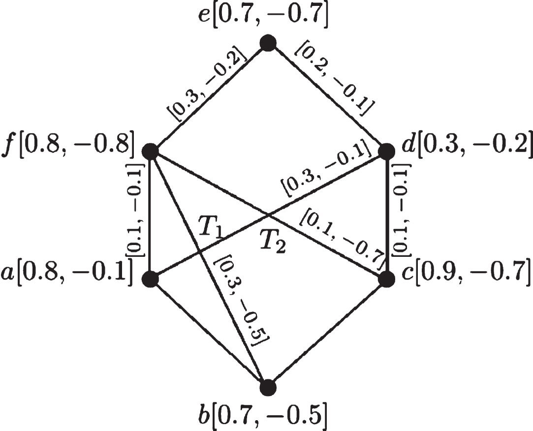
An example of very p-strong BFPG as well as very strong BFPG.
For the intersecting point T1, the edges (a, d) and (b, f) are intersected at T1, the positive-strength ( the positive-strength ( then the intersecting value at the point T1 is
For the intersecting point T2, the edges (a, d) and (c, f) are intersected at T2, the positive-strength ( the positive-strength ( then the intersecting value at the point T2 is
Therefore, the degree of planarity of the fuzzy graph shown in Fig. 2 is
Let 0 < c < 0.5 be a rational number. If
Obviously, for a specific value of c, a set of p-considerable edges is obtained and for different values of c, one can obtain different sets of p-considerable edges. Actually, c is a pre-assigned number for a specific application. For example, a social network is viewed as a BFG, where a social unit (people, organisation, etc.) is taken as a vertex and the relation between them is represented by an edge. The amount of friendship (measured within unit scale) is taken as positive membership value of the edge and similarly the amount of animosity is taken as negative membership value. Now for this network, if we choose c = 0.25, then we get a set of p-considerable edges, say C. This set gives a group of people who have some p-considerable amount (0.25 in this case) of relationship.
Similarly, the definition of n-considerable edges is given below.
The number of point of intersections between p-considerable edges and n-considerable edges can be determined from the following theorems.
In crisp sense, K5 and K3,3 cannot be drawn without crossing of edges. So, any graph containing K5 or K3,3 is non-planar, in conventional sense.
Let ξ = (V, E, A, B) be a bipolar fuzzy complete graph of five vertices where V = {a, b, c, d, e}.
From Theorem 1, it is known that the degree of planarity of a bipolar fuzzy complete graph is
Similarly, it can be shown that a bipolar fuzzy complete bipartite graph
Face of a planar graph is an important parameter. We now introduce the face of a BFPG. Face in a BFG is a region bounded by edges. Every face is represented by edges in its boundary. If positive membership values of all the edges in the boundary of a face are 1 or negative membership values of that edges are -1, then the face becomes a crisp face. If one of such edges is removed or has positive membership value 0 or negative membership value 0, the face does not exist. So the existence of a face depends on the minimum value of strength of edges in its boundary. A face in BFG is defined below.
Strength of faces in BFG belongs to [0,1]. If the strength of a face greater than 0.5, the face is called strong otherwise it is weak face. Every BFPG has an infinite region which is called outer face. Other faces are called inner faces.
Vertex and edge membership values of the BFPG considered in Fig. 3
F1 is bounded by the edges (v1, v2), (v2, v3) and (v1, v3), F2 is bounded by the edges (v2, v3), (v2, v4), (v3, v5) and has an infinite region (this face is an outer face), F3 is bounded by the edges (v1, v2), (v2, v4) and (v1, v4), F4 is bounded by the edges (v1, v5), (v1, v3) and (v3, v5).
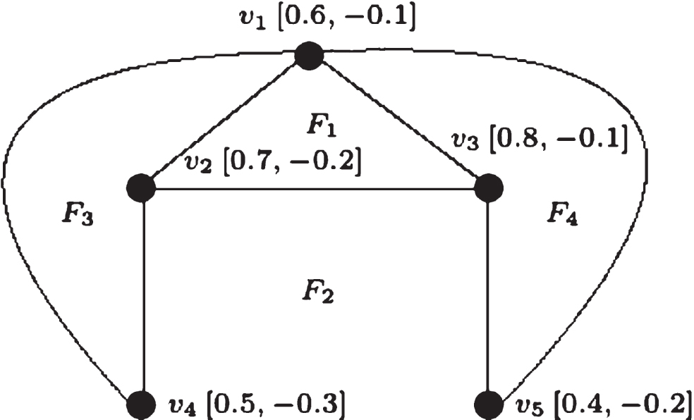
Example of faces in BFPG.
Strengths of all these faces are calculated and listed in Table 2.
Strengths of the faces of the BFPG shown in Fig. 3
From Table 2 it is observed that, F3 is a strong face. The face F3 is surrounded by very p-strong edges. Therefore a conclusion can be drawn that, every strong face is surrounded by either very p-strong edges or very n-strong edges.
In this section, we introduce the dual of a BFPG whose degree of planarity is 1. In bipolar fuzzy dual graph, a vertex corresponds to each face and there is an edge between two vertices if the faces corresponding to the vertices are adjacent by an edge. The formal definition is given below.
Between two faces F
i
and F
j
of ξ, there may exist more than one common edge. Thus between two vertices x
i
and x
j
in BFDG ξ′, there may be more than one edge. We denote
If there be any pendant edge in the BFPG, then there is a self loop in ξ′ corresponding to this pendant edge. The membership value of the self loop is same as to the membership value of the pendant edge.
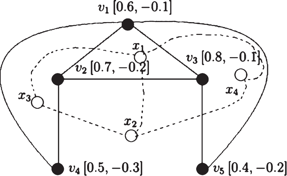
Bipolar fuzzy dual graph of a bipolar fuzzy graph.
Vertex x1 is corresponding to the face F1 which is bounded by the edges (v1, v2), (v2, v3) and (v1, v3). Therefore,
Vertex x2 is corresponding to the face F2 which is bounded by the edges (v2, v3), (v2, v4), (v3, v5) and has an infinite region. Therefore,
Vertex x3 is corresponding to the face F3 which is bounded by the edges (v1, v2), (v2, v4) and (v1, v4). Therefore,
Vertex x4 is corresponding to the face F4 which is bounded by the edges (v1, v5), (v1, v3) and (v3, v5). Therefore,
The edges of the dual of BFPG and their membership values are
The number of edges of two BFG ξ and ξ′ are same as ξ has only very p-strong edges. For each edge of ξ there is an edge in ξ′ with same membership value. ■
Image segmentation is one of the important step in partitioning any digital image. Also, image segmentation is used to recognize digital objects. Therefore, image segmentation is helpful process in computer vision, remote sensing, etc. The aim of image segmentation is to extrapolate the objects for different interest from background of the image. Images are segmented by different procedures. In this section, a methodology is described for image shrinking by segmenting each portions of an image by using BFPG.
An image is characterized by pixels and it has some homogeneous sections. It can be represented by a graph described below. Each pixel is represented by a vertex and its positive membership value (negative membership value) is determined by its intensity i.e. gray value (dullness or non-intensity). Two neighbouring pixels (vertices) are joined by edges. The positive membership value (negative membership value) of the edge is determined by the dissimilarity (similarity) value of the corresponding pixels (vertices). Several methods are available to measure the dissimilarity or similarity between two pixels. One of them is used to measure the edge membership values. Thus the entire image (see Fig. 5 for example) is converted to a BFG (see Fig. 6) where each coloured vertices signifies the corresponding segmented coloured portion of the image of Fig. 5. The edge membership values for the edges of the graph shown in Fig. 6 is given in Table 3. Obviously, this graph is a BFPG. Also, in the representation, no edges cross other. So the degree of planarity of the graph is 1 (then the graph is strong BFPG). The background of the image is represented by the unbounded face. The BFDG of this BFPG can be drawn by the method described in the Section 4 (see Fig. 7). The vertex and edge membership values of the BFDG shown in Fig. 7 is given in Table 4.

An example of a color image for image shrinking.
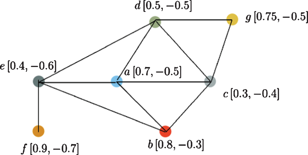
BFPG corresponding to the image shown in Fig. 5.
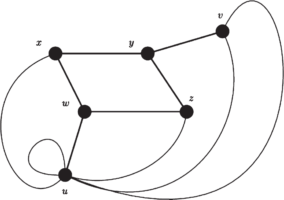
Corresponding BFDG of the BFPG shown in Fig. 6.
The edge membership values of the edges of graph shown in Fig.6
Vertex and edge membership values of the BFDG shown in Fig. 7
Now, we define some related terms such as edge and kernel shrinking.
Let ξ = (A, B) be a BFG and (a, b) be an edge. Suppose, this edge is shrinked, then a new vertex, say c, is created such that all the edges incident to a and b are now incident to c, and the edge (a, b) is removed from the graph. Also the positive membership value of the vertex c is given by σ P (c) = max {σ P (a) , σ P (b)}. The negative membership value of the vertex is given as σ N (c) = max {σ N (a),σ N (b)}.
If more than a pair of vertices are shrinked, then an extended shrinking method, called kernel shrinking is used. Suppose the edges (a, b), (a, c), (a, d), (a, e) are to be shrinked simultaneously. Also let, σ P (i) = m i , σ N (i) = n i , where i = a, b, c, d, e be given and all these edges are shrinked to a single vertex, say h. The positive membership value of the vertex h is given by max {m i , i = b, c, d, e} and negative membership value of the vertex is given by max {n i , i = b, c, d, e}. Note that the vertices b, c, d, e are merged to the vertex h.
Collection of some homogeneous pixels forms a homogeneous section. Two pixels or two homogeneous sections are said to be nearly homogeneous section if the difference between the membership values of the pixels or sections is less than some pre-assigned positive number. Nearly homogeneous sections (non-considerable edges) are shrinked in different levels and each level is obtained from its previous level. From Fig. 6, it is clear that an image is divided into some regions and a region is bounded by lines. In the BFDG, the edges are the boundary of the images.
Let us consider Fig. 8. In level 1 of the image pyramid, each pixel is represented as vertex. Two continuous homogeneous or nearly homogeneous pixels or sections are shrinked into a single section. This process is done by edge/kernel shrinking on the BFG. Also, by this process, the corresponding edges of the dual graph are removed. The final shrinked image is shown in the top level of the pyramid (see Fig. 8).
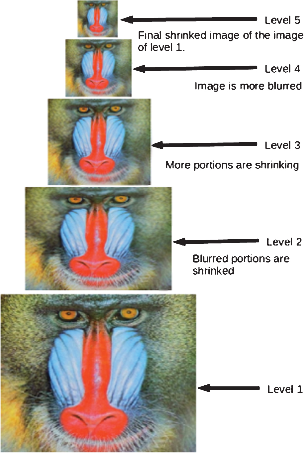
An example of image pyramid.
Suppose, in a city planning, city routes are to be so designed that the number of accidents should be minimized. Now, the number of accidents depends on many factors, like traffic system, road conditions, number of crossing between routes, etc. To solve this route planning problem, keeping in mind these factors, in a mathematical way, we convert the problem into a bipolar fuzzy graph model shown in Fig. 9.
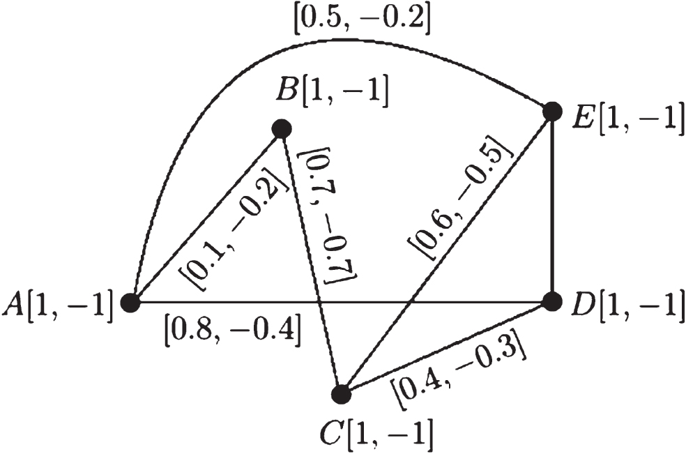
Bipolar fuzzy planar graph corresponding to a city route planning.
In this bipolar fuzzy graph consider routes as edges and vertices are the transporting points. As the transporting points has no contribution to this problem, the membership values for all the vertices are taken as [1, - 1]. The positive membership values of edges are assigned some grade between 0 and 1 depending on chances of accidents in the corresponding route. The negative membership values of edges are assigned some grade between -1 and 0 depending on traffic system available for that route. The gradation corresponding to traffic system is conceptually taken as negative since a better traffic system can decrease the chances of accidents. Thus, the membership values of the edges (A, E) and (C, E) are [0.5, - 0.2] and [0.6, - 0.5] respectively, which means the traffic system of (C, E) is more strong than (A, E) and the chances of accidents for the route (C, E) is more than (A, E). Now, our problem is to find how much this model is acceptable in the context of accident? For this, we compute the degree of planarity. After usual computations, the degree of planarity for this graph is approximately 0.30. Greater the degree of planarity means the chances of accident is less and vice-versa. So, we conclude that there are approximately 70% chances of accident.
This study describes the bipolar fuzzy multigraphs, bipolar fuzzy planar graphs, and a very important consequence of bipolar fuzzy planar graph known as bipolar fuzzy dual graphs. A new term “degree of planarity” is defined. This parameter characterizes a bipolar fuzzy graph in many ways. Several properties can be investigated on regular bipolar fuzzy planar graph, irregular bipolar fuzzy planar graph.