
Abstract
In multimedia English teaching, learners face such an indifferent computer screen without emotion and feel the fun of interaction and emotional stimulation, which will cause resentment and affect the learner’s learning effect. In order to improve the efficiency of multimedia English teaching, aiming at the lack of emotion in multimedia English education, this study proposes an intelligent network teaching system model based on deep learning speech enhancement and facial expression recognition. Moreover, this study uses emotional calculation as the theoretical basis and uses facial expression recognition as the core technology to judge and understand the emotional state by capturing and recognizing the facial expressions of online learners. In addition, this study has carried out experimental tests on the effect of the identification method of this paper and verified that the method has good detection effect on the real smile micro-expressions through two sets of experiments and can provide theoretical reference for subsequent related research.
Introduction
Online education is an educational method that uses multimedia computer technology and network technology to achieve optimal education. It is far superior to traditional education in terms of resource sharing and interactivity. However, because a key element of online education is the separation of teachers and students, the separation of schools and students, the teacher-student interaction in the online education environment is not carried out in real situations. However, the emotional communication that takes place is real. It cannot be denied that there is a real emotion between teachers and students because of the virtualization of network interaction. In the traditional classroom teaching environment, a teacher’s eyes, a sentence, an action will have an impact on the students’ learning [1]. In online education, teachers and students cannot perform face-to-face emotional communication. The emotional information brought by facial expressions, voices, and gestures is missing in the transmission process. The absence of all this emotional information will have an impact on the emotional interaction between teachers and students. On the one hand, it is difficult for students to feel the attention of teachers to them. Therefore, it is easy to produce confused and lazy emotions in learning. On the other hand, it is also difficult for teachers to understand the feelings of students and to effectively control the learning process of students [2].
Most modern online education only replaces conventional media with multimedia represented by computers and networks. It regards advanced information technology as a simple communication tool, uses network technology to carry out “textbook moving” or “electronic lesson” teaching, and publishes some textual teaching content or practice questions on the Internet. This kind of “electronic textbook” does not take advantage of the multimedia interactive technology, nor does it fully play the role of the network and lacks emotional incentives. The monotonous text information transmission replaces the colorful classroom teaching. The learner only sees the streaming textbooks similar to the textbooks but does not see the performance of the teacher’s emotional “emotional teaching role”. The interaction between the learner and the computer relies on only the keyboard and mouse. Not only does the computer not have visual functions, does not have language functions, and does not have auditory functions, and it does not have the ability to understand and adapt to people’s emotions or moods. When the learner faces such an indifferent computer screen without emotion for a long time and does not feel the fun of interaction and the emotional stimulation, it will cause resentment and affect the learner’s learning effect [3].
In this paper, aiming at the lack of emotions in multimedia English education, this paper proposes an intelligent network teaching system model based on facial expression recognition. It uses emotional calculation as the theoretical basis and facial expression recognition as the core technology. Moreover, this paper hopes to build an emotional computing model that can recognize facial expressions by means of related theories and techniques of emotional computing, especially facial expression recognition technology. By capturing and recognizing the facial expressions of online learners, judging and understanding their emotional state, and then giving corresponding emotional encouragement or emotional compensation strategies according to the learner’s specific emotional state, thus helping learners to compensate for the missing emotions in online learning to a certain extent. In addition, this article hopes to make a useful attempt to solve the problem of emotional loss in online education.
Related work
Foreign studies on facial expression recognition technology are relatively early, and Galbally J [4] first proposed that human expressions are mainly classified into seven types. These seven expressions are set to Happy, Angry, Surprise, Fear, Disgust, Sad, and Normal. This classification method is still used by a large number of researchers, and this classification method is also used in this paper. M. Suwa, N. Sugie, Xu Y et al. [5] conducted a series of studies on facial expressions in video. Peng X [6] and other people’s facial expression recognition system can identify four common expressions, namely happy, angry, surprised, disgusted. The recognition accuracy of the system is close to 80%. The system first determines the facial motion direction of the face through the optical flow, and then extracts the optical flow value of the local space into a feature vector. Finally, the facial expression recognition system is constructed according to the feature vector. In the 21st century, foreign researchers began to use more methods to analyze facial expressions. Yin X [7] and others used Gabor to study facial expressions. In order to reduce the influence of lighting and other factors on facial expressions, they preprocessed facial expression data. Moreover, they used the local features of the face as a benchmark and extracted the average Gabor wavelet coefficients as facial expression features, which were used to perform facial expression recognition. Lu J [8] and others proposed a new image retrieval algorithm, which expresses the facial expression features of the face by defining key modules and achieves a good recognition accuracy. K. Anderson, Mahmood Z [9] and others built the Facial Action Coding System (FACS). The study describes facial facial movements by depicting facial action units (AUs) and detects facial expressions by comparing the relationship between facial facial movements and expressions. Ding C [10] confirmed that the unsupervised learning and supervised tuning of neural networks can effectively improve the accuracy of neural networks. From then on, deep learning has become a hot topic for scholars. The huge breakthrough in deep learning has attracted the attention of top universities and research institutes, and they have gradually expanded their research investment in deep learning. Mahmood Z [11] people proposed two ways to improve the accuracy of facial expression recognition. One approach is to use polynomial parameters to describe time-independent original features. Another way is to use a combination of Support Vector Machine (SVM) and Hidden Markov Model (HMM) to build a classifier when using a classifier, which will increase the accuracy compared to using a support vector machine (SVM) alone. Nikitin M Y [12] designed a three-layer neural network. The neural network first uses the training set to train to obtain the model, and then uses the personal expression recognition database for retraining. It achieves a high recognition accuracy and can recognize the face expression in real time.
Target detection in behavior recognition
Background subtraction
Background Subtraction (BS) is a widely used moving target detection method. By pre-establishing the background model, it uses the training image to obtain the parameters of the model and uses the current image and the background image to reduce the brightness of the same position pixel to perform foreground target detection [13]. A frame background image is first selected or constructed, the background image is updated according to a certain background model, and then the difference image between the current image and the background image is calculated, and the difference image is thresholded to obtain a foreground target. The specific algorithm flow is shown in Fig. 1:
Flow chart of the Background Subtraction.
In the figure, f
k
(x, y) is the current frame, B (x, y) is the background image, I (x, y) is the grayscale image after the background difference, and R (x, y) is the image after binarization and connected domain detection.
The moving target is extracted by the difference between the current frame and the background image, the binarization processing, and the connected domain detection.
However, changes in the scene and light will cause the background to change every moment. Therefore, it is not advisable to select a frame with no moving target as the background from the video, and an adaptive background update model needs to be established. A more common approach is to use the image averaging model and achieve a weighted average of the image by assigning different weights to the current frame and the previously accumulated background. The specific method is as follows:
In the formula, B k (x, y) is the pixel value of the point (x, y) in the current background, C k (x, y) is the pixel value of the point (x, y) in the current frame, and Bk+1 (x, y) is the pixel value of the point (x, y) after the update. α is the update coefficient. The larger α is, the faster the background update is. The smaller α is, the slower the background update is. Therefore, its size should be set according to the actual situation.
The background subtraction algorithm is simple and easy to understand and has good real-time performance and can extract moving targets more completely. However, in the scene with large background changes, the detection performance is poor, and the pseudo-target is often generated. Therefore, further optimization is needed on the background modeling and updating methods [14].
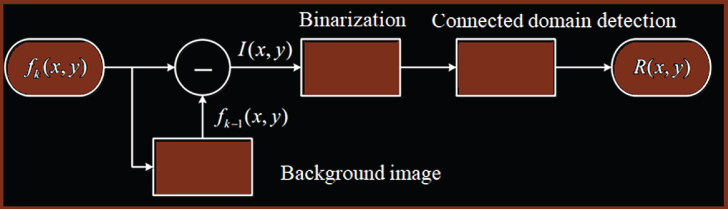
The interframe difference method refers to performing differential operation between consecutive image frames (between two frames or three frames), and subtracting the pixels corresponding to different frames to determine whether the absolute value of the gradation difference exceeds the threshold value to extract the moving target in the sequence image. The algorithm flow is shown in Fig. 2:

Flow chart of the interframe difference method.
In the figure, f
k
(x, y) is the k-th frame, fk-1 (x, y) is the k–1-th frame, I (x, y) is the grayscale image after the difference, and R (x, y) is the binarized image.
The variation region of the moving object in the video image is detected by the difference calculation between two adjacent frames. For static targets, such as a stationary background behind the target, I (x, y) is zero. For a moving target in the scene, I (x, y) is not zero.
In order to better display the foreground target of the motion and remove the influence of noise on the motion foreground, the differential image will be binarized and connected domain detected.
In the formula, T is the threshold for binarization.
On the basis of the interframe difference method, the adjacent three frames of images are differentiated as a group to detect the moving target. The flowchart of the specific algorithm is shown in Fig. 3:

Flow chart of the interframe difference method (three frames).
In the formula, f k (x, y) , fk-1 (x, y) , fk-2 (x, y) is a continuous three-frame image, and I1 (x, y) , I2 (x, y) is a differential image calculated by two adjacent frames. The specific algorithm process is as follows:
The difference image I1 (x, y) , I2 (x, y) is obtained by the difference between the two adjacent frames of the video frame. Then, binarization processing and connected domain detection are performed on the calculated difference image.
The two binarized images calculated for each pixel point are ANDed to obtain the detected foreground target image.
Whether it is the interframe difference method or the improved three-frame difference method, the advantage is that the algorithm is simple, the operation speed is fast, and the light can be adapted to a certain extent to a certain extent, and the adaptability to the dynamic environment is good, and the influence of the target shadow is small. However, the shortcoming of this method is that the moving target area cannot be completely extracted, the positioning is not very accurate, and it is too dependent on the moving speed of the target [15]. When the target moving speed is large, voids and ghosts often appear.
The optical flow can be thought of as the instantaneous velocity field produced by the movement of pixels with grayscale on the image plane. Horn and Schunck assume that the image region is continuous and steerable both spatially and temporally, which is considered an important constraint in the calculation of optical flow. For an image sequence, we assume that the luminance value of a pixel (x, y) in the image at time t is I (x, y, t). u (x, y) and v (x, y) represent the motion components of the optical flow at the point (x, y) in the x and y directions, respectively. In a sufficiently small time dt, point (x, y) moves to point (x + dx, y + dy), dx = udt, dy = vdt. According to the assumption that the brightness is constant, that is, the corresponding pixel points in each frame along a certain motion trajectory curve have the same gray value, that is, the brightness of the corresponding point on the image is unchanged, we can obtain:
The above formula is developed by the first-order Taylor formula to obtain the following formula:
In the formula, O (∂2) is a higher order trace of dx, dy, dt second or third order, which can be ignored. Taking into account the speed relationship,
In the formula, I x , I y , I z represents the gray value of the point. The partial derivatives of I (x, y, t) in the x, y, t direction can be obtained from the image sequence. V = (u, v) is the velocity field, and ∇I = [I x , I y ] T is the spatial grayscale gradient of the image pixel point (x, y). Equation (12) is the optical flow constraint equation, or the basic equation of optical flow, which represents the relationship between the grayscale spatial gradient of the image and the velocity of the optical flow. In the optical flow constraint equation, u and v are both unknowns and only one constraint equation, so the optical flow cannot be uniquely determined. Additional constraints are needed to determine u and v.
The basic idea of the introduced constraints is that the optical flow should be as smooth as possible and the smoothing constraint E s is minimized:
According to the basic equation I
x
u + I
y
v + I
t
= 0 of optical flow, the optical flow error E
c
is minimized to obtain:
The solution to the optical flow field can then be translated into a solution to the following problem:
The minimization equation is solved, and the optical flow vector [16] is obtained by calculating the adjacent gray image of two frames.
For the n × n region adjacent to the pixel, if the motion trend of the pixels is assumed to be the same, the following equations can be established:
The above equations can be expressed as a vector form:
By the least squares method, the equation can be solved and the direction and size of the optical flow vector can be obtained. However, when the above-mentioned n × n window contains more than two edges, the L-K optical flow method can ensure that the matrix is an invertible matrix, thereby ensuring that the optical flow defining equation has a solution. Therefore, the calculation process of the L-K optical flow method needs to combine the corner information and the edge information, and the optical flow vector obtained in this way is the sparse optical flow vector [17].
Forward neural network
As a computational model, the forward neural network is composed of multiple levels of neurons. Each level consists of multiple neurons connected. The structure of the forward neural network is shown in Fig. 4 [18].
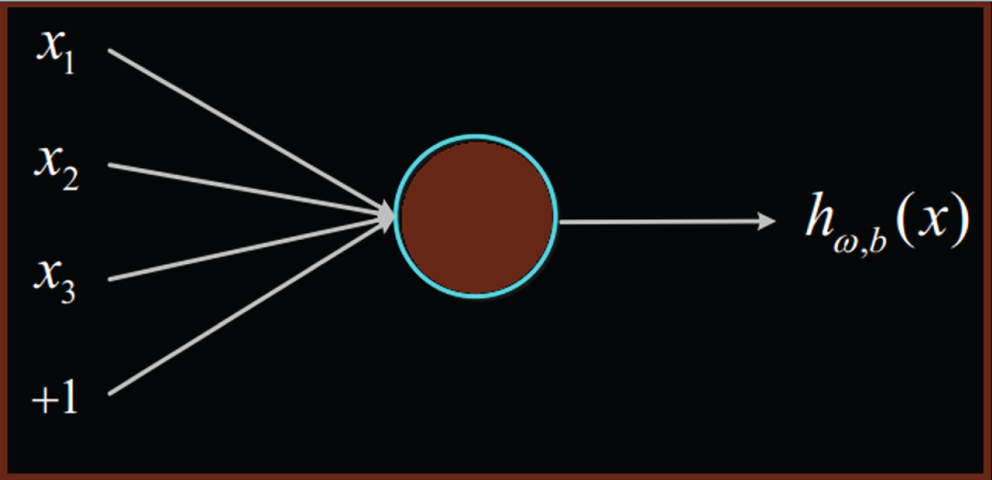
Single neuron structure.
The neuron has three inputs (x1, x2, x3) and one output hω,b (x), respectively, and the computational relationship is:
In the formula, x represents the input vector, W is the weight vector of the input, b is the offset, and function f : R → R is the activation function.
The structure of the forward neural network is shown in Fig. 5. The network model can be determined by the number of specific network layers and the number of neurons in each layer. The learning process of the entire neural network is based on constantly adjusting the weights and bias coefficients of the neurons. Generally, a forward neural network has an input layer for receiving data to be processed, and then followed by multiple hidden layers or no hidden layer, receiving the output of the upper layer, after calculation by multiple neurons, the last layer Is the output layer [19].
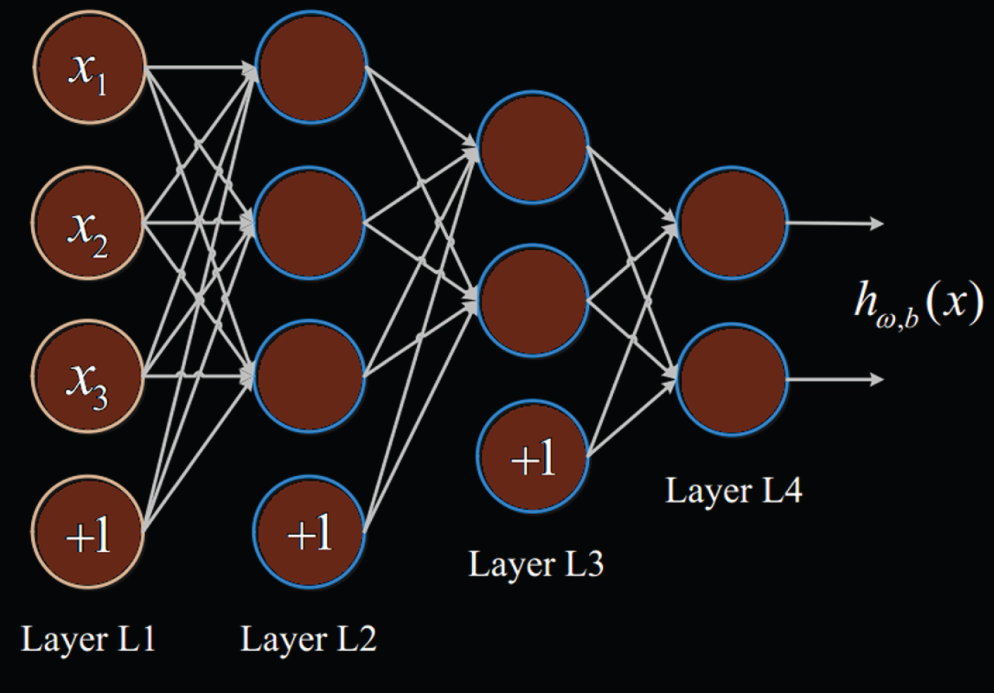
Structure of the forward neural network.
The Convolutional Layer is also a feature extraction layer. It convolves the data of the upper layer by a plurality of convolution kernels of different sizes, thereby obtaining different two-dimensional outputs. The calculation formula is as follows:
In the formula, x is a two-dimensional input vector, ω ij is a convolution kernel of size i × j, b is an offset, y mn is the output of size m × n, and function f is the activation function. The function of the convolutional layer is to convolve the output of the upper layer by multiple convolutional kernels to obtain a plurality of new two-dimensional outputs. The two-dimensional output calculated by convolution is called a feature map.
This idea of connecting local information is also inspired by the structure of the visual system in biology. The neurons of the visual cortex receive information locally, that is, these neurons respond only to the stimulation of certain regions. The local perceptual characteristics of the convolutional neural network are shown in Fig. 6:
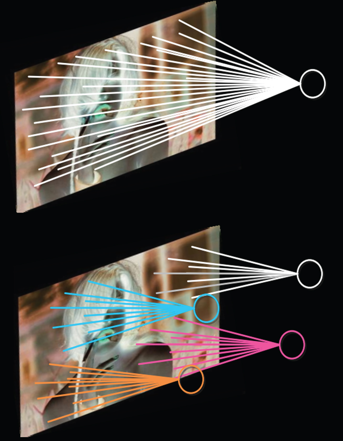
Full connection mode (top) and local connection mode (bottom).
While reducing the amount of calculation, the robustness of the network output to displacement and deformation is also improved. The formula for the pooling operation in a certain area is:
In the formula, xm×S1+i,n×S2+j is the pixel value of the input two-dimensional image at m × S1 + i, n × S2 + j, and y mn is the output obtained after pooling. The pooling layer can reduce the amount of computation of the network, and makes the network have certain invariance to the translation and scaling of the object, so that the network is robust. The pooling layer is actually down-sampling on different channels. The down-sampling process of different channels is independent of each other. The process of pooling operation and convolution kernel are similar to sliding on the image. However, the pixels that are drawn by the pooling layer do not overlap each other, and the step size can be determined to determine the size of the feature map after the pooling operation. As shown in the right half of Fig. 6, the four pixels in each S1 × S2 region are combined into one pixel by calculating the average value, then added by the weight ω and the offset coefficient b, and finally the two-dimensional feature map is obtained by the excitation function f. Therefore, the pooling layer also plays the role of extracting features again.
Support Vector Machines (SVM) is a two-class classification model whose basic model is the linear classifier with the largest interval in the feature space. We assume that the hyperplane is ω · x + b = 0, and |ω · x + b| can relatively represent the distance of point x from the hyperplane. In general, the distance between a point and the separation hyperplane can indicate the degree of confidence in the classification prediction. For a hyperplane (ω, b) of a given training data set T, the function interval for the sample point (x
i
, y
i
) is defined as:
The function interval can indicate the correctness and certainty of the classification prediction. However, when choosing to separate hyperplanes, the equal scaling of ω and b does not change the hyperplane, but the function interval is changed by a multiple, so the unique solution cannot be found and is not suitable as the objective function of the classifier. Therefore, the normal vector ω of the hyperplane needs to be normalized, so the geometric interval is introduced:
In the formula, ∥ω∥ is the L2-norm of ω. The maximum interval separation hyperplane can be expressed as
The Softmax classifier generalizes the loss function of logistic regression to multi-classification problems. When there is a task of class k, and the training set has a sample of m numbers, and the input is an n-dimensional vector, the training set can be expressed as:
In the formula, y(i)∈ { 1, 2, ⋯ , k } is the label and x(i) ∈ Rn+1 is the sample. The Softmax classifier will calculate the probability that each sample belongs to k classes:
This forms a k-dimensional output for each sample, and the form of the calculation function is as follows:
In the formula,
The goal of training the Softmax classifier with the training set T is to find the appropriate parameters to minimize the loss function of the classifier. The commonly used loss function is as follows:
The smaller the value of the loss function, the more accurate the result of classifying the training set by Softmax.
AlexNet’s network structure is shown in Fig. 7. The entire network consists of 12 layers of input layers, including 1 input layer, 5 convolutional layers, 3 pooling layers, and 3 fully connected layers. Compared with LeNet, AlexNet has achieved good results in the ImageNet object classification task, which makes the convolutional neural network return to people’s field of vision.
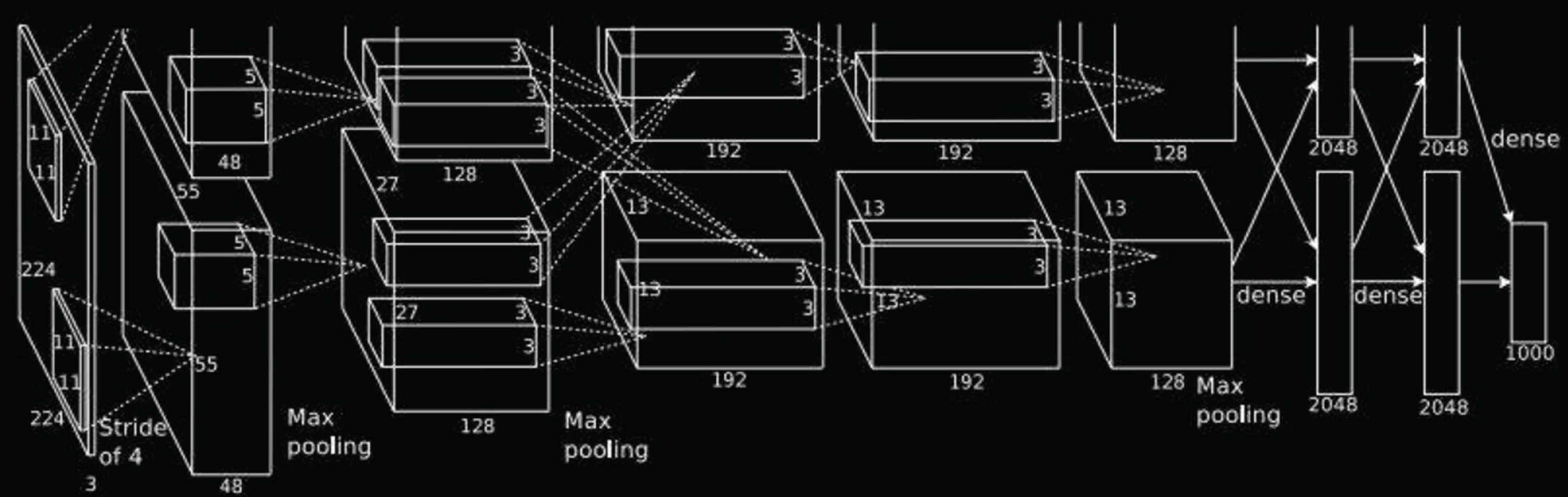
AlexNet network structure diagram.
ZFNet is a convolutional neural network designed by Matthew D. Zeiler and Rob Fergus in 2013. ZFNet’s greatest contribution is to visualize the feature map by deconvolving and de-pooling convolution operations and pooling operations in the network to analyze the evolution of the various layers of the convolutional neural network and potential problems, and further optimize the network.
GoogLeNet is the 2014 ILSVRC Challenge champion. Under the premise of not increasing the demand for computing resources, the structure of the neural network is improved, and the depth of the entire network is improved, thereby improving the effect of network training. Although increasing the network width and depth can improve the network performance to a certain extent, the number of parameters of the deeper and larger network model will increase greatly, which will easily lead to over-fitting of the network. Therefore, GoogLeNet uses a sparse alternative to a dense connection, and proposes a structural model of the network in the Inception network, as shown in Fig. 8.
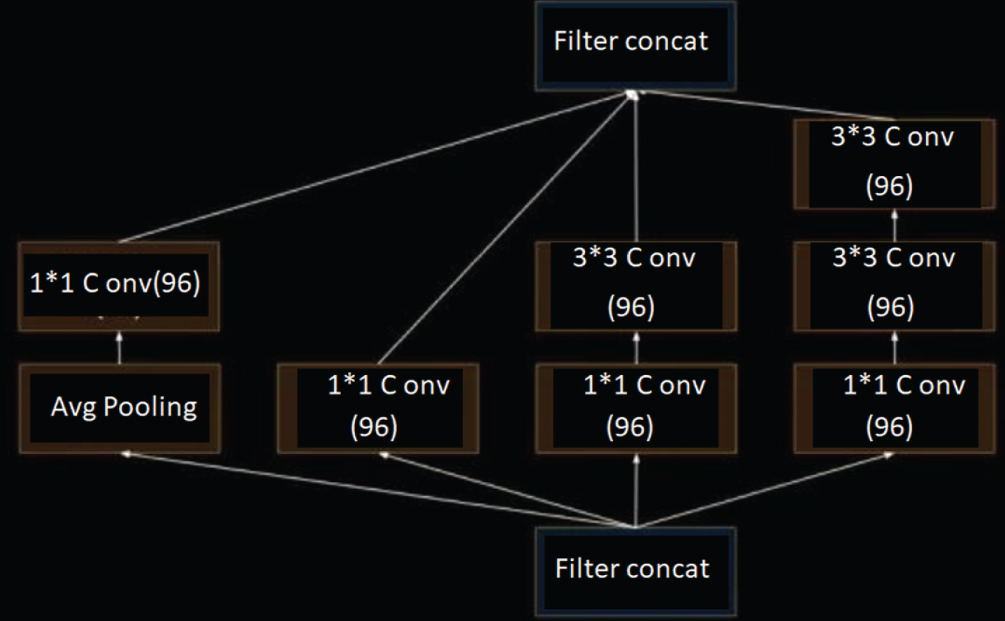
Inception V1 structural model.
The purpose of the Inception structural model is to cover the coefficient structure as an approximately dense structure by finding the optimal local sparse structure. The main theoretical idea of the Inception model is to represent the probability distribution through a large sparse network structure and to construct an optimal structure by analyzing the statistical correlation of the activation state of the nodes in the previous layer, and to aggregate the neurons with higher output correlation. GoogLeNet’s overall network structure has 22 layers, and the depth has increased significantly compared to AlexNet, but the number of network parameters has been reduced by 12 times compared to the number of AlexNet. When the large-scale image classification is performed based on the GoogLeNet network model, the classification accuracy rate is higher.
ResNet is a residual network structure proposed by the MSRA He Kaiming team in 2015 and is the champion of the classification task of the ImageNet competition that year. The depth of the network is a non-optical flow network that optimizes network performance. The two adjacent frame images are superimposed and input into the network, and the number of channels is 6, and the entire network has a total of 9 convolution layers. The 6 convolutional layers have a step size of 2, and the convolution kernel decreases with the depth of the convolution. The convolution kernel of the first convolutional layer is 7 × 7, the convolution kernel of the next two convolutional layers is 5 × 5, and the convolution kernel after that is 3 × 3, and the entire network does not have a fully connected layer, as shown in Fig. 9.
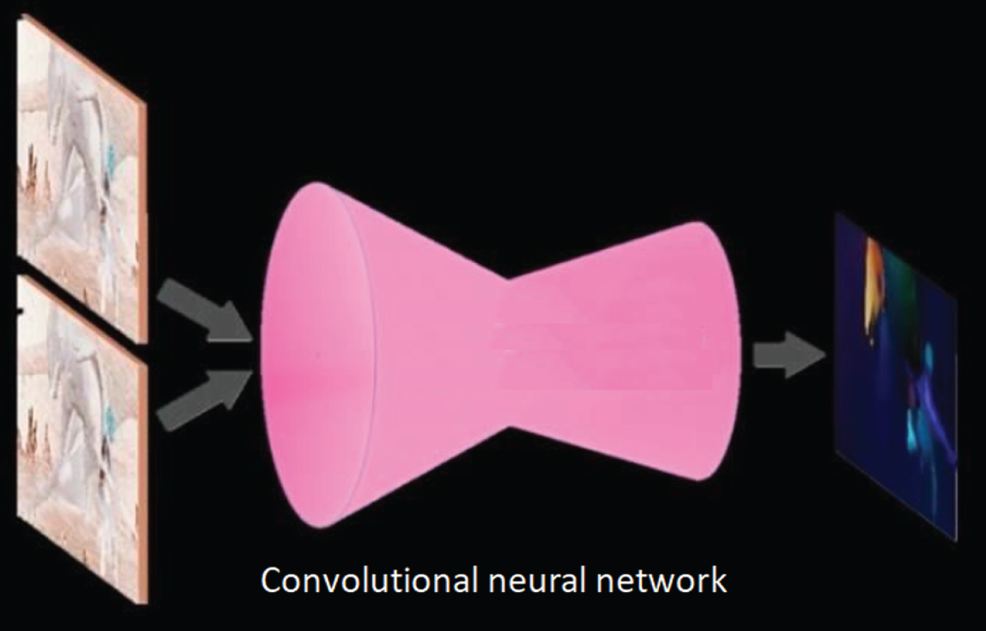
End-to-end convolutional neural network.
The optical flow network consisting only of convolutional layers is shown in Fig. 10, and the other is to process two input images separately. The features of the two independent images are shown in Fig. 11. The two adjacent frame images are processed separately, and the respective feature maps are obtained by the respective convolutional neural networks, and the relationship between the two feature images is found through the correlation layer. The two feature maps calculated by the two convolution channels are
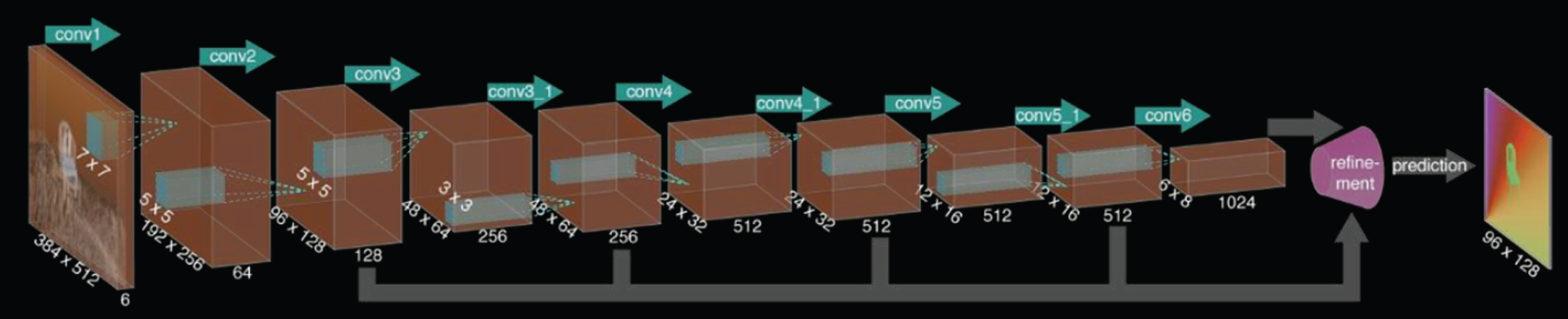
Optical flow network consisting only of convolutional layers.
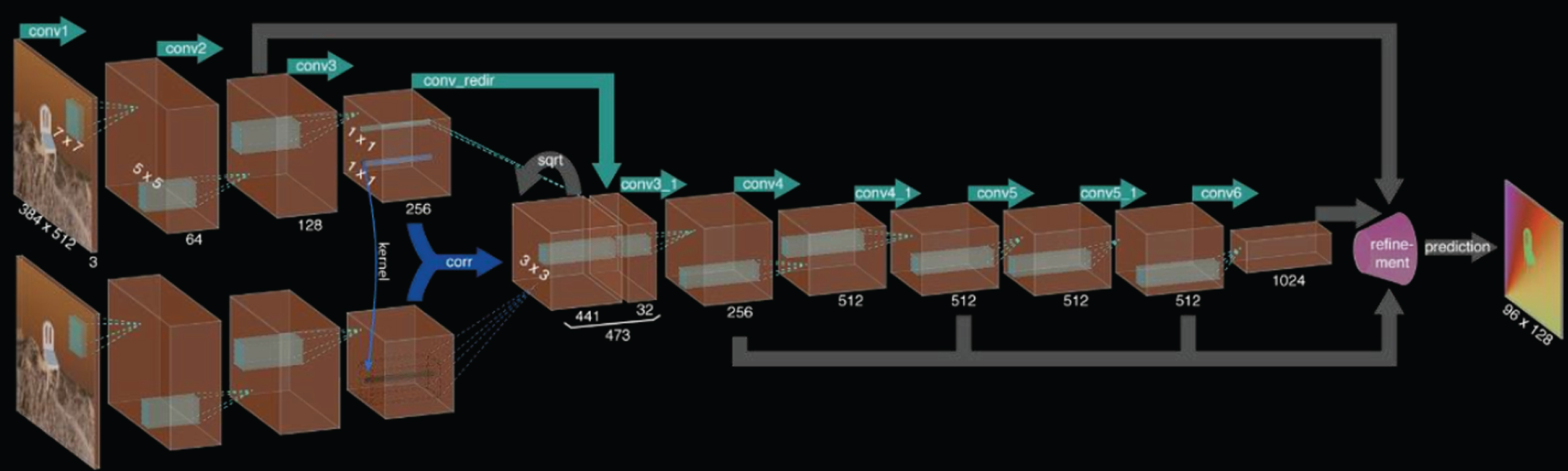
Optical flow network added to the relevant layer.
At the end of the entire optical flow network, an important extended portion is included to extend the compressed optical flow image to be equal in size to the input image. As shown in Fig. 12, the extended part of the network is a thin convolutional layer that maps the coarse features to a high-resolution optical stream image, and the upper convolution is applied to the feature map and is connected to a part of the corresponding feature map. This can preserve high-level and coarser feature maps and can also pass information on low-level networks well. In order to refine the details of the optical flow image, the image boundary is calculated, and the smoothing coefficient is replaced by α = exp(- λb (x, y) k ). b (x, y) represents the boundary strength resampled between the corresponding scale and pixels. This amplification method is more computationally complex than simple bilinear up-sampling, but because of the advantages of the variational method, the optical flow field is smoother and more accurate.
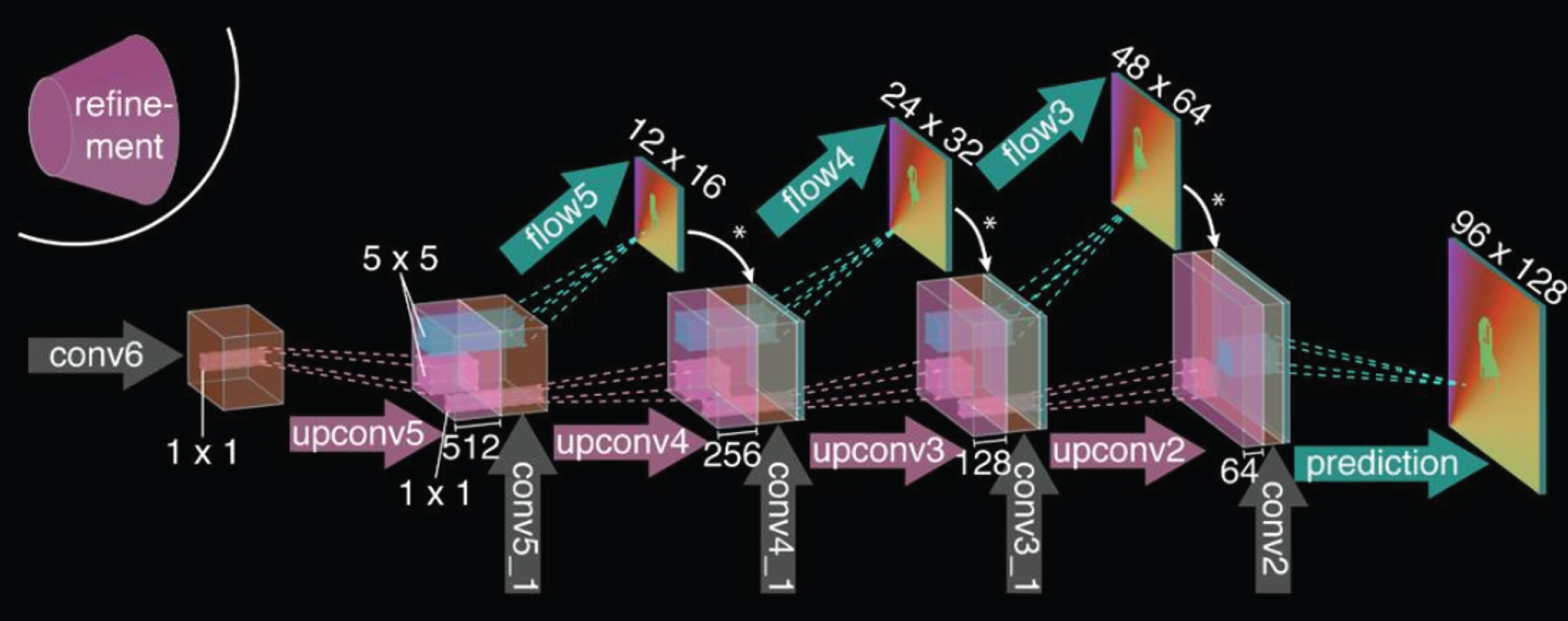
Coarse feature refinement is mapped to a high-resolution optical flow image.
The proposed optical flow network has transformed the method of optical flow estimation. The optical flow network directly learns the concept of optical flow through data. However, the effect of the above optical flow network on small displacement and actual data cannot be compared with the traditional method. Eddy Ilg and Nikolaus Mayer of the University of Freiburg proposed a combined optical flow network with multiple optical flow networks for optical flow estimation. While grasping the large displacement between video frames, it accurately estimates the details in the optical flow field and solves the problem of noise artifacts. Compared with a single optical flow network, it greatly improves performance in practical applications such as motion recognition and motion segmentation.
The operating platform of this experiment is the Windows 10 operating system. The Python language is used, so the platform needs to install a Python-related environment. The database used in the experiment was the CASME2 micro-expression database. Because there are less expression samples of non-real laughter in the CASME2 micro-expression database, the camera is used to collect the laughter expressions of 10 students as experimental test data, and the expression recognition framework OpenCV and deep learning framework Keras are used.
In the CASME2 micro-expression database, most of the expressions about laughter are micro-expressions generated under natural induction, so most of them belong to the real expression range of laughter. Therefore, the main purpose of this group of experiments is to test the accuracy of the detection of real expressions in this method. Figure 13 and Fig. 14 show the related expressions of laughter expressions and some experimental samples in the CASME2 micro-expression database. Since the database is a micro-expression database, the movement of the laughter expression is small.
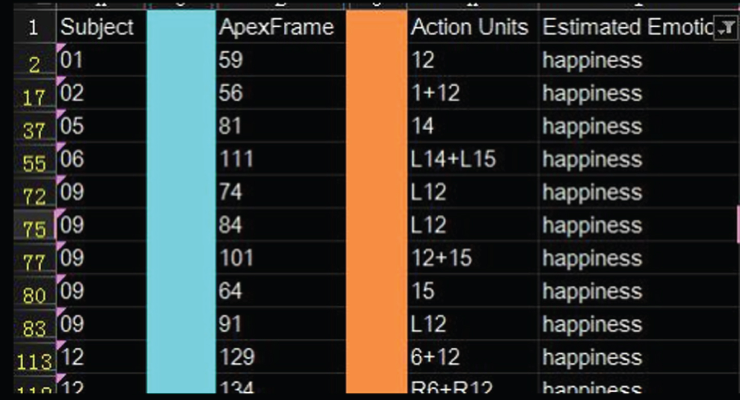
Laugher expression information in CASME2.
Part of a sample of laughter expressions in CASME2.
In view of the lack of non-real laugher expression samples in the previous group experiments, In this group of experiments, the experiment of real and non-real expressions generated by 10 students was carried out by natural induction method to test the accuracy of real and non-real expression recognition in this method. Figure 15 shows the collected sample expressions of some of the students, all of which are initial calm expressions.
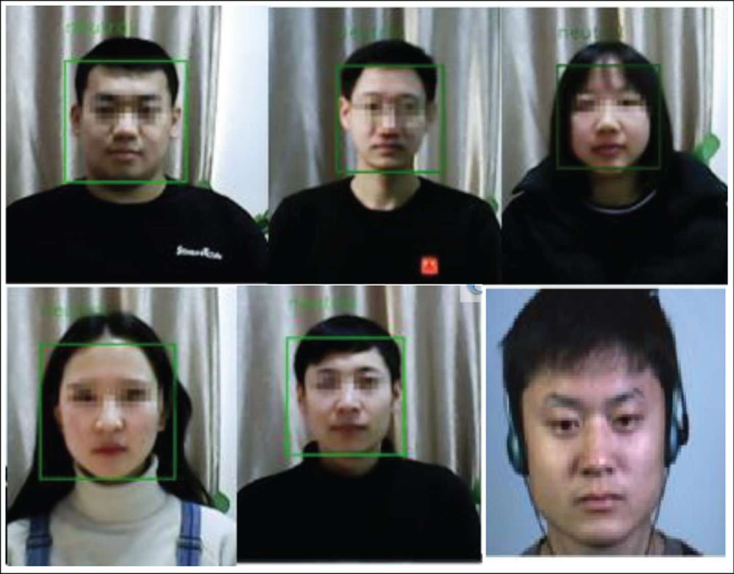
Samples of expressions of some students.
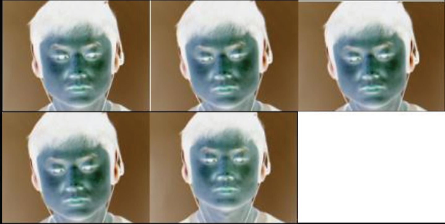
In this experiment, CASME2 has a total of 32 micro-expression video samples of laughter. The ratio of expression training samples and recognition samples used is 1:1, and each video sample in the training sample uses 10 corresponding training pictures. In the 16-segment laugh recognition video of CASME2, a total of 12 videos recognized the real laughter expression, and the recognition results in the other 4 videos were neutral faces. Figure 16 is a screenshot of some experimental results.
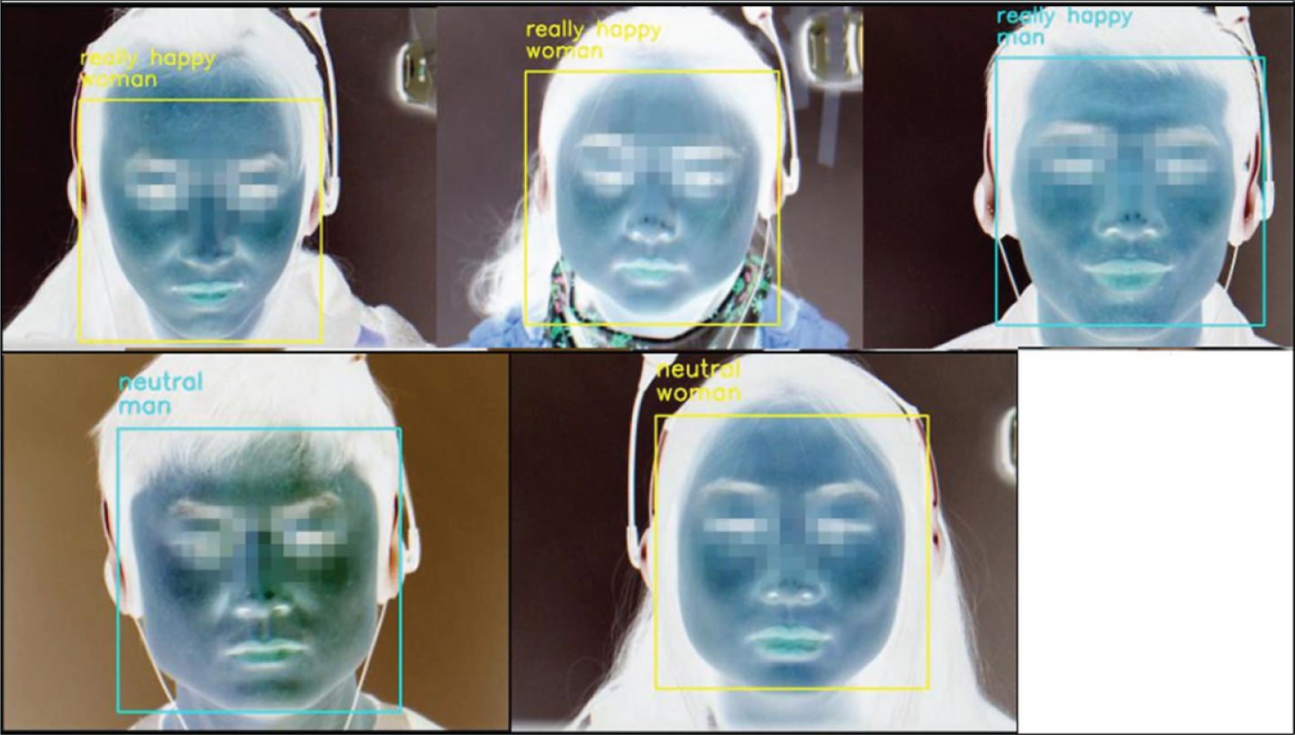
Screenshot of some experimental results in the experiment.
The recognition result of the real laugh of some students.
Among them, the upper part is the result of the recognition of the real laughter expression, which has 12 segments, accounting for 75%. The next part is the result of the unrecognized real laughter expression, which consists of 4 paragraphs, and the result is neutral face, accounting for 25%.
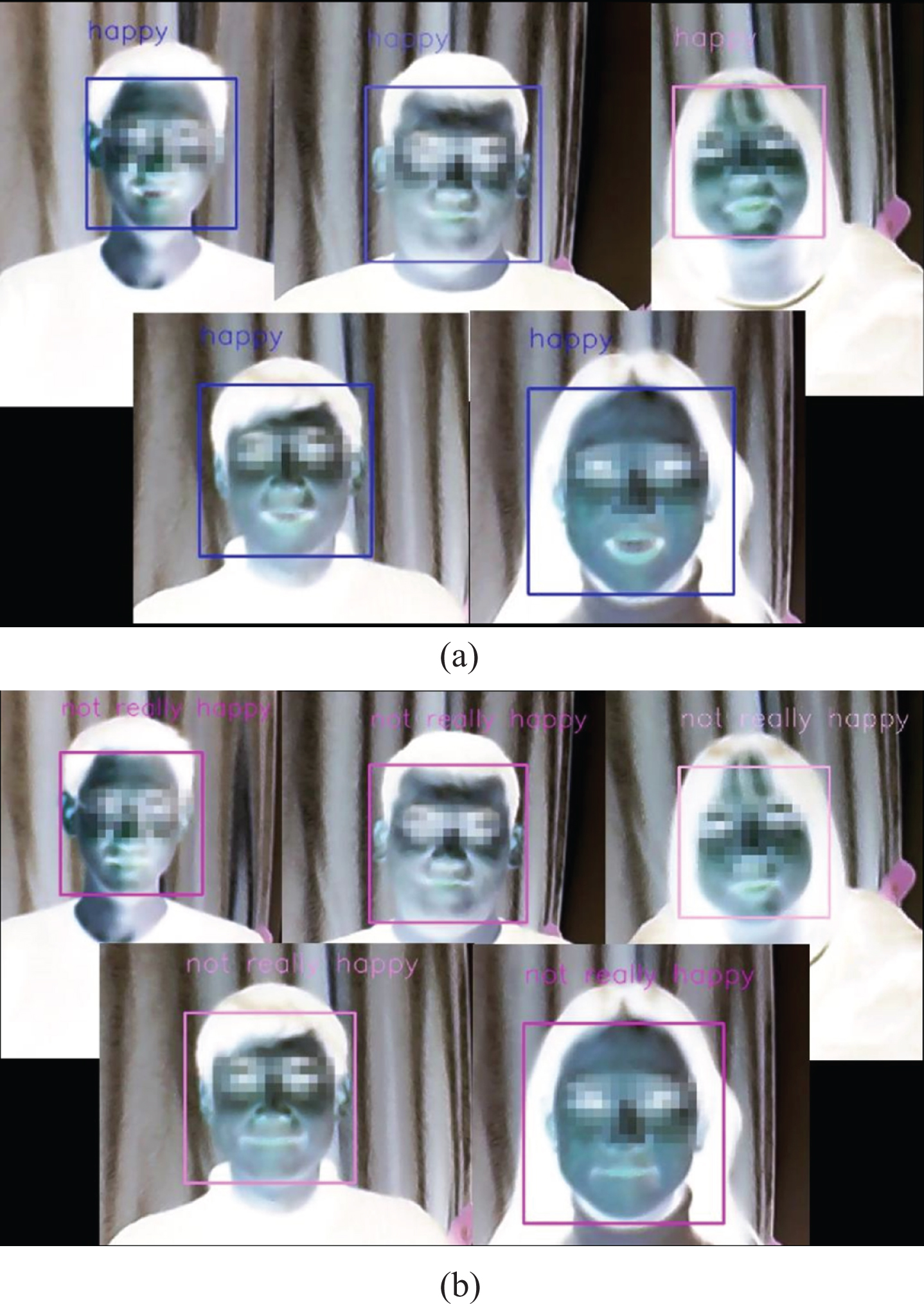
Referring to the natural induced method, 10 students were selected to perform real-time recognition of the camera. In the experiment, the effective expression time of each classmate was 15 seconds, which included both real laugh and unreal laugh. In the experiment, the average duration of the effective expression produced by each classmate is 15 seconds, which includes both real laughs and non-real laughs. The result of the discrimination is happy, which means that the corresponding laughter expression is generated by the corresponding students, and the result of the judgment is not really happy, which means that the meaning of the corresponding students is a non-real laughter expression
The recognition results of the 10 segments of the experiment were processed according to the Facial Behavior Code System (FACS) analysis and the experimental personnel’s data feedback. The experimental results are shown in Table 1. The detection rate in the table refers to the proportion of expressions displayed by the experimenter that can be detected (in this experiment, it shows that the experimenter shows neutral, true laugh or unreal laugh). The missed detection rate is the proportion of the results of the failure to detect the expression displayed by the experimenter (in this experiment, the expression of the expression displayed by the experimenter is not recognized). The recognition accuracy rate refers to the proportion of the correct result of the recognition of the expression category in the detected case, and the recognition false detection rate refers to the proportion of the result of the recognition of the expression category error in the detected case.
Statistical table of the experimental results
From the table, the average detection rate is 78.3% %, and the average recognition accuracy is 77.8%. The identification data samples used in this experiment are not the same as the training samples, and the micro-expression data samples of laughter are less. Therefore, this experiment mainly verifies the recognition effect of the real emotions of the laughing expressions in the general expressions, and the verification results show that the algorithm recognition effect is obvious.
Aiming at the lack of emotion in multimedia English education, this paper proposes an intelligent network teaching system model based on facial expression recognition. It uses emotional calculation as the theoretical basis and facial expression recognition as the core technology. This paper hopes to build an emotional computing model that can recognize facial expressions by means of related theories and techniques of emotional computing, especially facial expression recognition technology, and to judge and understand the emotional state by capturing and recognizing the facial expressions of online learners. ding Based on the deep learning-based speech enhancement algorithm and expression localization, the algorithm designed in this study is used for multimedia English teaching analysis, and the experiments are carried out for verification analysis. This study introduced the experimental environment and the framework used, and explained the experimental samples used by the two experimental groups. Next, the experimental results of the identification method of this paper were tested. Through two sets of experiments, it not only verifies that the method has a good detection effect on the real laughter micro-expression, but also proves that the method has higher accuracy for the recognition of students’ general expressions in multimedia English teaching.