
Abstract
Attribute and class noises are the two important sources of Corruptions (noise) contained in real-world datasets which may deteriorate data interpretation and accuracy. Class noise has potentially serious negative impacts compared to attribute noise, however, the existing major class noise detection methods are not able to address this problem efficiently. To overcome issues related to detection and the elimination of class noise, we suggest a new noise filtering approach able to identify and remove class noise, called Multi-Iterative Partitioning Class Noise Filter (MIPCNF). Since there is no single filter that consistently outperforms its counterparts in all database types and in different levels of noise, our approach relies on an algorithm in which several rounds of class noise detection are performed on different partitions of the data using several classifiers. Therefore, we use different filtering strategies: iterative noise filter, partitioning filter and ensemble-based filter. The experimental results, on 14 real-world datasets, and statistical analysis, show that our method is not only overcoming the higher noise but also over-performing latest class noise detection and elimination strategies in different levels of noise.
Introduction
Classification is a process which extracts automatically knowledge from a set of data during a learning phase, then uses that knowledge in order to group the data into homogeneous classes during a prediction phase [1]. However, real - world databases often contain a large amount of noises that may deteriorate data classification accuracy. Indeed in classification, a model is built from labeled examples, in order to predict the class for new examples. Obviously, both the learning phase and the model obtained will be negatively affected, if the data used to train this model are corrupted due to the presence of noise. As a consequence, the final model will be less accurate and more complex. Noise can be divided into two different types [16]: attribute noise and class noise. Attribute noise refers to errors in attribute values and class noise (also called labeling errors) pertains to misclassified instances or instances with different wrong class labels. Moreover, other irregularities such as outliers may raise, which might not be noisy points but only special cases of regular examples. Outlier detection [1–4, 56] and anomaly detection [7–10] methods can be used for class noise detection.
Class noise elimination has become increasingly as common pre-classification task due to the fact that labeling data with high reliability are often expensive and difficult to obtain. In [14, 17], it is shown that the class noise is potentially more harmful, in terms of instances misclassification, than the attribute noise, which underlines the importance of taking into account this type of noise. This unsatisfactory classification quality is explained mainly by two reasons: Firstly, for a given instance, there are many characteristics or attributes whereas while only one class label is associated with the same given instance. Secondly, the importance of the attribute is, in general, variable; whereas the number of attributes is always big in case of class labels because the latter guide the learning towards the desired classification rule.
Effectively, many research have suggested that in most cases, eliminating instances which contain attribute noise is not always correct and, because many other attributes of the instance may still contain valuable information [14]. However, eliminating class noise will seriously improve the classification accuracy.
The causes of class noise are various and it is often impossible to know precisely. Class noise is human and can have several potential causes: The subjective nature of the classes involved in the labeling task. The information provided to the operator may have poor quality or may be insufficient to determine the true label of a given instance [22]. Therefore, the user can therefore just assume or guess the class that he thinks is suitable for this instance. The operator has uncertain knowledge in labelling instances. Additionally, since label collection is a costly task and time-consuming, using non-expert operators for an easy and cheap labeling is gaining a growing interest between researchers.
Intentional errors such as those considered in [23, 24], for example, in mail filtering tasks, a malicious user may introduce class noise deliberately to mislead the spam classifier.
Other examples can be noticed such as misunderstanding of the mechanism used to label instances, or simply lacking of attention (e.g. accidental clicks), or even making perceptual errors due to fatigue.Other method proposed in [25] aimed to design a locally optimal estimator against the fault and noise signals.
The main disadvantage of class noise is the decrease in classification accuracy [38, 57]. Indeed, class noise not only affects badly the predictive capabilities of the learned model, but also increases its complexity [15, 55]. Bi and Jeske [26] show that class noise increases the error rates and biases the parameters of the normal discriminant and, in lesser extent, the logistic regression. The presence of class noise can also affects the classification performances of the k nearest neighbors (kNN) classifier [27, 28].
In the scholarly literature, a major issue related to class noise detetection is that no single filter that consistently outperforms the others, in all database types and in different levels of noise,. For example, in Ensemble Filter (EF) approach, noise is eliminated in a single round, which can ignore a lot of class noise.
According to several studies, we report some issues in this context: The problem of selecting an appropriate classifier according to each problem. The wrong choice of the learner, which may not have the suitable bias for performing some cases. The problem of the dataset size limitation especially in case of large datasets.
In this paper, we propose a new algorithm aimed at overcoming all the problems cited bellow for detecting and eliminating class noise. The importance of dealing with this type of noise raises from the fact that class noise is potentially more harmful than attribute noise. Our proposed algorithm will be denoted Multi-Iterative Partitioning Class Noise Filter (MIPCNF). Our approach relies on an algorithm in which several rounds of class noise detection are performed on different partitions of the data. Iterative-partitioning filter enhancing classification accuracy has been adopted. Thanks to parallel processing, our approach can handle large dataset effectively. Therefore, we improve the performance of the class noise elimination based on combination of several filtering strategies.
Additional strength points of our methodology are as follows: Our solution over-performs latest class noise detection and elimination strategies in different levels of noise. Our solution allows selecting the suitable classifiers based on the characteristics of the dataset. The algorithm is scalable because it allows filtering large and/or distributed datasets. The experimentations, which are carried out over different large data in multiple iterations, show that our approach overcomes the higher noise. This implies that the results are efficient and reliable.
The rest of the paper is organized as follows. Section 2 presents related works. Section 3 describes our proposed approach. Section 4 discusses the results of different experiments. Finally, Section 5 enumerates some useful conclusions.
Related work
This section presents brief survey of existing works and the inspiriting driving this paper. Some authors propose support vector regression in primal using squared pinball loss which play an important role in diminishing the effect of noise [40]. The detection of class noise is not trivial. Many methods are proposed for detecting, deleting, or re-labeling mislabeled instances (class noise) with varying degrees of success. Instead of removing instances that are likely to be mislabeled, another solution would be to have them re-labeled by an expert, as proposed in [41, 42]. However, depending on the applications, this may prove to be too expensive. There are some studies, which have been done to evaluate the impact of both removing and relabeling techniques on noise detection using classification filtering algorithms [15]. In several research such as [43, 44], it has been observed that the simple elimination of mislabeled instances is as effective as their re-labeling. In the other hand, an approach which tackle the noisy multi-class problem [18], analyzes the usage of decomposition strategies to deal with this problem.
Melville et al. [29] have presented an average-case analysis of the kNN classifier. When k is optimized, the consequences of class noise are reduced except in the case of adding a large amount of class noise. The optimal value of k depends on both the percentage of class noise in the data and the number of training examples. For small and clean training sets, 1NN classifiers are usually optimal. However, the optimal number of neighbors (k) increases with the added number of class noise, even n the case of small training sets. This seems natural since class noise is particularly affecting 1NNclassifiers [15].
Several studies have shown that boosting is affected by class noise [30, 31]. In particular, AdaBoost (adaptive boosting algorithm) tends to spend too much effort to handle class noise [30]. During learning phase, classifiers are successively trained and the weights of instances, that are judged as class noise,are increased at the next step. Hence, in the last step of the classification, AdaBoost increases the weights of mislabeled instances in order to overfit the class noise issue [32, 33]. Class noise can affect not only the learning performance but also the complexity of learned models. For example, [34] the size of decision trees may increase depending on the presence of class noise, which makes the learning process overly complicated. This is confirmed experimentally in [35]. Similarly, the study in [33] shows that the presence of class noise increases the number of nodes of decision trees induced by C4.5 classifier, while the classification accuracy is reduced. Reciprocally, in [35, 36] it is shown that removing class noise can reduce the complexity of SVMs [15]. This highlights the need to implement techniques that eliminate class noise or reduce their impacts.
To deal with this issue, several kinds of solutions have been proposed, such as those based on confidence measures associated with thresholds [11], nearest neighbors [2], prediction of the classifier [3], and density based methods [4]. In the approaches using confidence measures such as distribution of the probability, the instances can be declared as noise when the computed measure is bigger than a predefined threshold. Authors in [12] present a method based on nearest neighbors. They classify an instance x using k Nearest Neighbors (kNN). This instance will be affected to a class C if at least k instances, belonging to this class, are among the k nearest neighbors of x. Otherwise, it will be considered as a class noise. Another example of detecting noise using prediction of the classifiers is proposed in [5], a support vector machine (SVM) is used to predict labels. The same method is actually used with neural networks [13].
Some machine learning algorithms could also detect noise. However, the main function of these algorithms is to find clusters instead of detecting noises. Consequently, many errors can be produced. In the other hand, noise filter is a common approach to deal with noisy datasets; the instances detected as noisy by the filter are simply removed [56]. The most common class noise filtering strategies are briefly described in the following: Classification Filter (CF) [45]: CF is a simple noise filtering approach. It splits the training set into n subsets. One single classifier is used for each subset. The examples which are misclassified by a base learner are then eliminated from the training dataset. The major drawback of this approach is that the decision is taken from only one single classifier. Consequently, this may lead to an erroneous prediction. Ensemble Filter (EF) [35]: EF classifies the training data using a set of classifiers. Then, the results are combined using a voting scheme. Therefore, the class noise is removed from the training data. The main disadvantage of this type of filter is that the whole dataset is handling in one hand which can be difficult in case of large datasets. Iterative-Partitioning Filter (IPF) [20]: The Iterative- Partitioning Filter builds only one base learner in multiple iterations until a given stopping criterion is reached. In each iteration, the training dataset is first partitioned into n subsets and one base classifier is built over each of these subsets. Then, the misclassified instances are eliminated (using voting scheme) and a new iteration is started. The fact that class noise is eliminated using only one base learner presents the drawbacks of this type of filter. According to the hypothesis that collecting predictions from different classifiers could provide a better class noise detection than collecting information from a single classifier [14]. The Iterative Noise Filter based on the Fusion of Classifiers (INFFC) [46]: INFFC consists on tree main steps. First, a preliminary filtering is applied using a classification filter to eliminate class noise in the current iteration. This first filtering allows reducing the influence of class noise in the next steps. Then, another filter (CF) is built from the partially clean data result of the preliminary filtering. The results of this step are two sets: clean and the detected class noise. Finally, class noise is eliminated if it exceeds a computed noise score. As least common filters we describe the following approaches, which use one base classifier (KNN) to eliminate class noise in different ways: Multiedit (ME) [47]: Training data are partitioned into n folds. k-Nearest Neighbor classifier is applied from the part x considering the part(x + 1) mod n as training dataset and the mislabeled examples are eliminated. This process is repeated until no examples are removed. Nearest Centroid Neighbor Edition (NCNE) [48]: This is a modification of ENN to identify and eliminate class noise, which consists of removing every example misclassified by the k nearest centroid neighbors (k-NCN) rule. Edited Nearest Neighbor (ENN) [49]: The examples which have class label different from that of the majority of its k nearest neighbors are removed. This is the main idea of this algorithm. All k-Nearest Neighbors (AllKNN) [50]: Varying the number of neighbors between 1 to k, the k-NN rule is applied k times. When all the values of k have been considered, the misclassified examples are discarded from the training set.
We will use all the filters above in our experiments to compare the performance of our approach with that of these filters (Section 4). The parameters with which each filter works are detailed in the Table 1.
Parameters for the noise filters
Parameters for the noise filters
MIPCNF: Multi-Iterative Partitioning Class Noise Filter
In this paper we propose our own class noise filter called Multi-Iterative Partitioning Class Noise Filter (MIPCNF), which allows for detecting and eliminating class noise iteratively using a set of classifiers to each sub-dataset. Our process of class noise elimination can be summarized in the three following steps: Firstly, we divide the training dataset into subsets. Secondly, the ensemble based filter is appliqued for each subset in several rounds. Finally, we combine the classifier’s prediction using a voting method to detect class noise. A scheme of our proposal MIPCNF is shown in Fig.1. Our class noise filter process is inspired by INFFC.
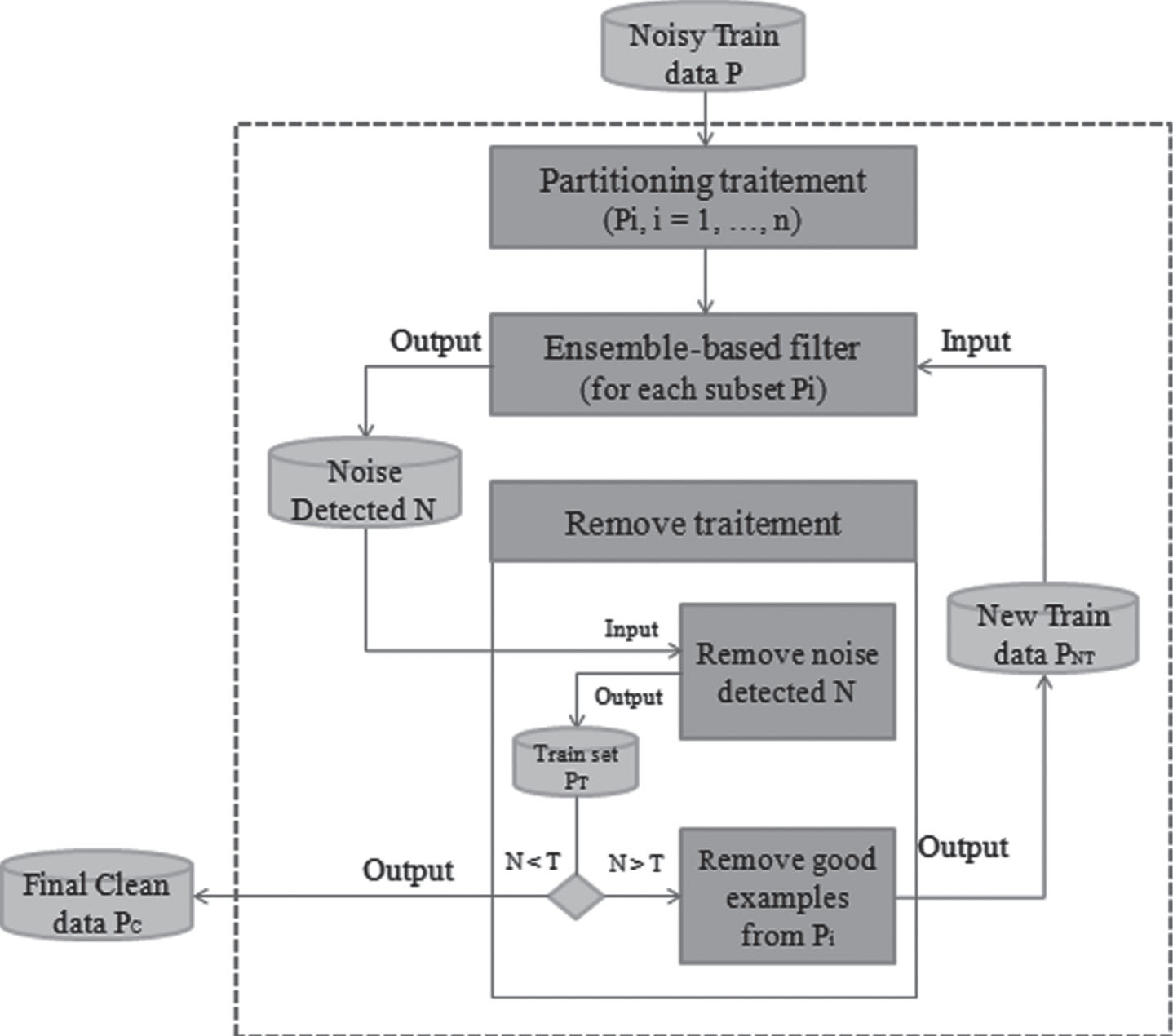
Architecture of Multi-Iterative Partitioning Class Noise Filter.
The components of our architecture are:
Partitioning data: This step consists on dividing the data into equal subsets in order to make parallel treatment; this may be beneficial in case of large data [53, 54].
Ensemble-based filter: An ensemble of classifiers is applied to each subset instead of a single classifier. Then, the partial outputs are combined into a single prediction using a voting method. The idea behind that is collecting predictions from different classifiers could provide a better class noise detection than collecting predictions from a single classifier. This diversity is one of the key to this approach. In the other hand, the simultaneous use of several classifiers makes it possible to combine the advantages without cumulating the disadvantages.
Verification process: In current iteration, we remove the identified misclassified examples. If the detected noise exceeds predefined threshold, a certain portion of good examples are also removed from the subset. Then a new iteration is started, and new Ensemble based Filter is applied using partially cleans data. The process will be iteratively repeated until the criteria are satisfied. The benefit of eliminating good examples [11] is that it can reduce the dataset size. Therefore, the classification process may be faster in the next iteration. The main advantage of eliminating noise in multiple rounds is providing the possibility to avoid the detected class noise in the new iteration. The detailed algorithm of our filter is represented in Fig. 2. The parameters used are described in Table 2.
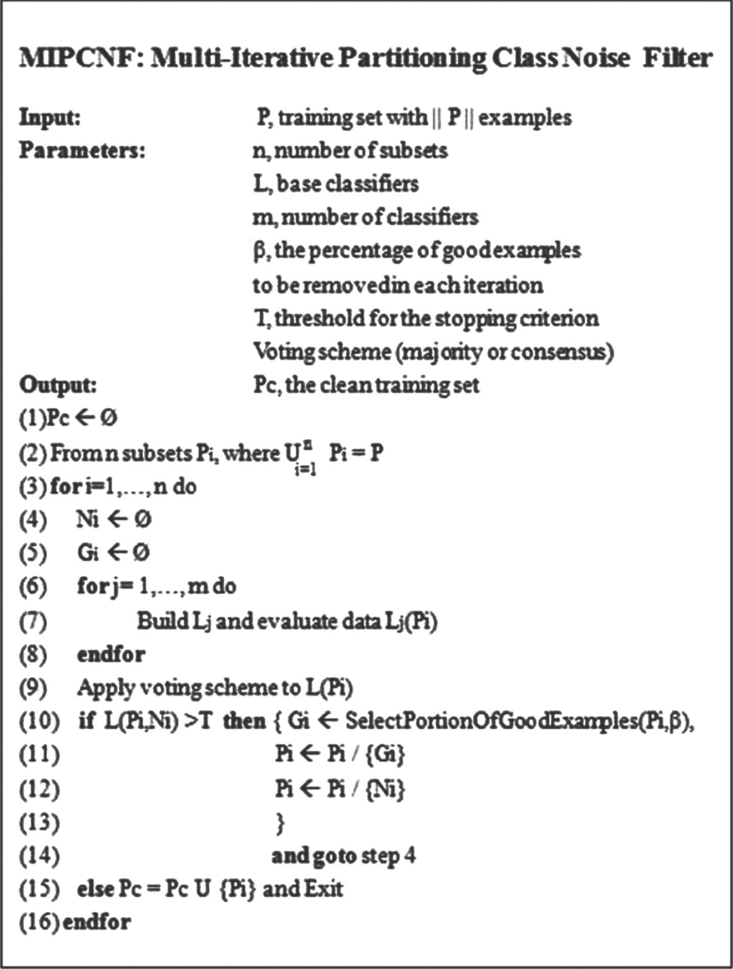
Algorithm of Multi-Iterative Partitioning Class Noise Filter.
Description of parameters used in the proposed noise filter
The difference between our filter and the INFFC by which we were inspired is presented below: INFFC algorithm seems to be too time consuming. Indeed, learning the whole dataset in one time is sometimes inadequate with large datasets. Hence, in some cases, the datasets cannot be handled at one time by the model. The partitioning filter adopted by our filter, described by Zhu et al. [16], tries to overcome the problem of the dataset size limitation. In our approach, the training dataset is first partitioned into subsets, small enough to be processed by a classifier. Another advantage of our filter compared to INFFC, is that we remove portion of good examples in each iteration. Thereby, the dataset size is reduced, allowing the induction learning schemes run faster in the next iteration. The experimental results reported in the next section demonstrate the effectiveness of our filter.
There are three main aspects to consider when comparing the time required for filtering of MIPCNF to that of the other ensemble-based filters considered in this paper (INFFC, EF and IPF): iterative elimination, partitioning of the training sets and the use of noise score.
The most significant difference in time complexity of MIPCNF with respect to INFFC is the computation of the noise score used by the latter (which is not used by neither MIPCNF, EF or IPF), which is mainly based on the usage of the k-NN classifier. Thus, even though INFFC might be slower than other ensemble-based filters, such as MIPCNF, EF and IPF (mainly due to the computation of the noise score).
The increase in the overall time complexity of the noise evaluation strategy used by MIPCNF with respect to EF and INFFC is due to two main causes: its iterative elimination of noisy examples (which is not used by EF, but it is by IPF and INFFC), and the internal partitioning of the training set to identify the noisy examples (which is not used by INFFC, but it is by IPF and EF).
The resulting computational complexity of our algorithm (MIPCNF) is O(n +Kn2), where n is the number of instances in the dataset and K is the number of the classifiers used. The running time taken by IPF can be estimated to be O(n2) + O(n) (for IPF we have K=1), it has approximately the same time complexity as our method. The running time of INFFC depends on the kNN complexity used into calculation of the score, the complexity of k-NN is of O(n. m), where n and m are respectively the number of attributes and the number of examples in the training set. So the overall time complexity can be close to O(n2) + O(n. m). The time complexity of EM is K h O([n. m]/h), where K and h are respectively the number of classifiers and the number of partitions, assuming K and h constants the overall time complexity can be further simplified to O(n. m). Compared to our method, this algorithm is faster.
However, the time is not the most important aspect to be considered since it is only required once. The main goal of our proposal is to enhance the classification accuracy, in our future work we will try to minimize the computational cost of our approach.
Experimentations
This section presents the details of our experimental study using a large collection of real-world datasets.
First, Section 4.1 describes the datasets used. Section 4.2 presents the parameters and the methods used by our algorithm. Then, Section 4.3 describes the experimental results as well as some statistical analysis, including comparative study with other well-known filters found in the literature in different noise levels. The description of the influence of some parameter in classification accuracy is also discussed.
Datasets
We have evaluated our noise elimination strategy based on the 14 numerical datasets taken from the KEEL-Dataset and UCI repositories [51, 52]. These datasets provide a good representation of different characteristics: numbers of samples are ranges from 101 to 58000 dimensionalities from 4 to 60 and number of clusters from 2 to 10. Balance: Balance dataset contains 625 examples that model the psychological experiments with three possible outcomes. It predict which way a scale is tipped or if it’s balanced. Each example is classified as having the balance scale tip to the right, tip to the left, or remain exactly in the middle (balanced). Car: This dataset represents a collection of the records on specific attributes on cars donated by Marco Bohanec in 1997. It was derived from simple hierarchical decision model. The car evaluation dataset contains 6 attributes: Buying, Main, Doors, Persons, Lug boot and Safety. Dermatology: This dataset contains 366 examples of dermatology cancer occurrences, it was found on OpenML - dermatology. It contains 33 attributes, 6 of which are psoriasis, seboreic dermatitis, lichen planus, pityriasis rosea, chronic dermatitis, and pityriasis rubra pilaris. Ecoli: This data set contains information of Escherichia coli (protein localization sites). It is a bacterium of the genus Escherichia that is commonly found in the lower intestine of warm-blooded organism. The dataset consists of with 336 proteins sequences labeled according to 8 classes. Ionosphere: This data set contains radar data collected by a system in Goose Bay, Labrador. The targets were free electrons in the ionosphere. It contains 351 examples, each using 33 continuous attributes. Divided in two classes, ‘Good’ radar returns are those showing evidence of some type of structure in the ionosphere, and ‘Bad’ radar returns are those that do not. Iris: This dataset aim to predict flower type of the Iris plant species: Setosa, Versicolor, Virginica. It includes 150 examples of flowers characterized by 4 attributes (sepal length, sepal width, petal length, and petal width), classified on 3 classes of 50 instances, where each class refers to a type of iris plant. Monk: This dataset aim to predict class based on planned distributions. The dataset consists of all 556 examples and 6 nominal attributes: 2 with 2 discreet values, 3 with 3 discreet values and 1 with 4 values. New-Thyroid: This dataset represents the diagnosis of thyroid whether it is hyper or hypofunction. It contains 215 examples and 5 attributes, used to classify 3 classes of thyroid function as being over function, normal function, or underfunction. Penbased: This datasets is about Recognition of Handwritten Digits. It consists of 10992 exmples and 16 attributes, describing the 10 written digits 0,...,9. Hence, there are 10 classes. All taken values are integer values between 0 and 100, inclusive. Pima-diabetes: This database was made by National Institute of Diabetes and Digestive and Kidney Diseases. The objective of the dataset is to diagnostically predict whether or not a patient has diabetes. There are total 768 examples using 8 attributes (6 discrete and 2 continuous). There are 2 unevenly distributed classes, 500 examples for class 0 and 268 instances for class 1. NASA Space Shuttle: This Real-life dataset is a fairly large compared to the others. This is a complex classification dataset that deals with the positioning of radiators in the Space Shuttle. NASA Shuttle control database is quite large and consists of a total of almost 58000 vectors. Each instance is described by 9 continuous attributes (namely, time, Rad Flow, Fpv Close, Fpv Open, High, Bypass, Bpv Close, Bpv Open, and class code) and is assigned to one of 7 classes. Splice: Splice junctions are points on a DNA sequence. The problem posed in this database is to recognize, given a sequence of DNA, boundaries between exon and intron. This DNA data-set contains 3190 examples with 60 attributes, representing a sequence of DNA bases. WDBC: Wisconsin Database of Breast Cancer, it contains 569 examples with 357 benign and 212 malignant cases. Each instance is described by an index, diagnosis, and 30 real-valued attributes. Zoo: The purpose for this dataset is to be able to predict the classification of the animals. It consists of 101 animals from a zoo. There are 16 attributes with various traits to describe the animals used to classify animals into seven types: Mammal, Bird, Reptile, Fish, Amphibian, Bug and Invertebrate. The majority of classes are distributed in well separated regions in the projection.
Table 3 summarizes the main characteristics of these datasets, organized according to their number of examples #EX, number of attributes #AT and number of classes #CL. The examples containing missing values were discarded out the datasets. In order to control the amount of noise in each dataset and verify how it affects the noise filtering methods. We inject different levels of classification noise in the data sets by replacing labels of 0%, 5%, 10%, 15%, 20%, 25%, and 30% examples of each dataset. For each dataset and noise level, we have 7 levels of noise which means 105 datasets. All experiments were carried out in 5-fold cross-validation. For each of the 5 runs, the data set was divided in a training set (80%) and a test set (20%). The train data are partitioned into 5 equivalent folds, 3 classifiers are build for each subsets. Hence, a total of 25x3 runs for 105 datasets will be preprocessed with our approach and other 7 noise filters resulting 63000 executions from which the results obtained are analyzed in this paper. Other experiments are also conducted in order to discuss the influence of some parameters in classification accuracy.
Datasets specification used in the experimentation
Datasets specification used in the experimentation
Among the broad suite of classifiers available in the literature, three classifiers were selected to use them in our algorithm (C4.5, SVM and logistic). This selection is according to the study presented in the next section (section 4.3.3). Table 4 summarizes the parameters used for these classifiers.
Parameters used for the classifiers used in our experimentation
Parameters used for the classifiers used in our experimentation
The threshold T (used in our algorithm) is equal to 1% of the size of the original training dataset E (i.e., T= ||E|| x 0.01). In addition, the percentage of good examples removed from the training set at each round is β = 50%.
In this work, all algorithms were implemented using java and the WEKA 3.6 data mining toolkits with its default values.
This experimental study aims at analyzing the effectiveness of our proposed architecture using large collection of real-world datasets. We investigate his robustness in different levels of class noise comparing with others recent approaches. We also varied some parameters to know the most suitable ones that allow us to have the higher classification accuracy. Note that the most difficult step in this work is the implementation of this algorithm as well as the learning phase using 14 different types of datasets, it take time, effort and concentration.
Comparison between our filter and the existing noise filter methods
We compare the robustness of our filter with 9 other filters proposed in the literature (described in section 2), according to the filter accuracy in different levels of noise. The accuracy formula (1) used to calculate the performance of the proposed filter is calculated using confusion matrix. In following formula, TN (True Negative) referred as correctly rejected samples, TP (True Positive) referred as correctly identified samples, FP (False Positive) referred as incorrectly identified samples and FN (False Negative) means incorrectly rejected samples.
The result is presented in Table 5 and Fig. 3. The best results at each noise level are highlighted in boldface. For each dataset we apply three base learners (SVM, Logistic and C4.5) in different levels of noise.
Classification accuracy of each noise filters in different levels of noise (best results are remarked in bold)
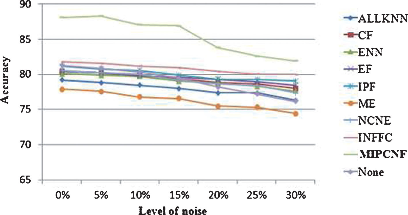
Classification accuracy of each noise filters in different levels of noise.
As it can be observed, our noise filter MIPCNF gives the best results at all noise levels (5% to 30%), including clean dataset (0% of noise). It gives a good result in some largest datasets (penbased, shuttle,...) as well as small ones (iris, zoo, monk,...). From the experimental results it can be also seen that MIPCNF presents a high level of accuracy compared to other state-of-the-art competitors. Indeed, the results of INFFC followed by IPF and EF are also remarkable, but remain below those of the MIPCNF. ME and AllKNN have the lowest results, they can be considered the worst filters.
In our system we execute the procedure for multiple iterations. Noise elimination will stop when the stopping criterion is reached: T= X.0.01, where X is the size of the training dataset.
We compare the prediction accuracy of our filter using Pima dataset for three different threshold values in different levels of noise. The obtained results are depicted in Table 6 and Fig. 4.
Influence of the threshold value on the prediction accuracy using using the Pima dataset
Influence of the threshold value on the prediction accuracy using using the Pima dataset
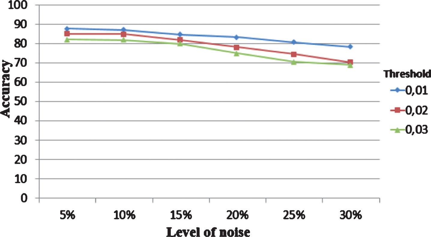
The impact of the threshold value on the prediction accuracy.
From the Table 6 and Fig. 4 we can notice that when we have threshold equal at 0.01 we got the higher accuracy compared to the others value of threshold. Indeed, in order to reach the stopping criterion we should add more iterations which means more precision. At high threshold values (in percentage) we reach the stopping criterion only in few rounds. Our experimental results indicate that when the noise level is relatively low, the results obtained are basically good enough compared to the existing methods. However, when the noise level goes high, more iteration is needed until the number of identified class noise in each round is less than the threshold.
There are several basic learners in datamining that can be used for noise detection. In our study, we select five learners, the most common to detect class noise: C4.5, SVM, Logistics, NaiveBayes (NB), RandomForest (RF). In this section, we compare the prediction accuracy for the Pima dataset based on the combination of three classifiers. With these five classifiers, we have 10 possible combinations of three classifiers.
The experimentation results (Table 7 and Fig. 5); allows us to conclude that the combination of these three classifiers (C4.5, SVM and Logistic) is the most recommended one to apply in our case.
Comparison between classifiers combinations according to the classification accuracy using Pima dataset with 30% of noise and a threshold T = 0.01
Comparison between classifiers combinations according to the classification accuracy using Pima dataset with 30% of noise and a threshold T = 0.01
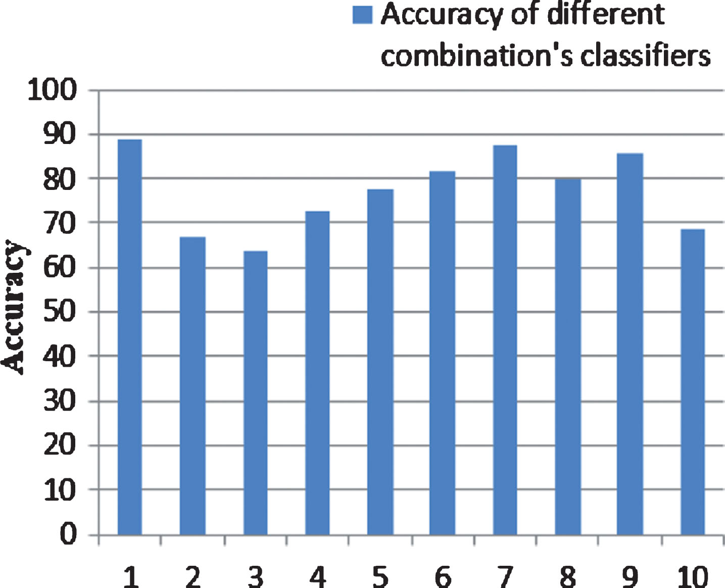
Comparison between classifiers’ combinations according to the classification accuracy.
In case of classification using a combination of classifiers, an instance is classified as noise using a vote on the various classifiers prediction. Different elementary combiners are compared in this section according to the classification accuracy, including the product, min, max, median, average rules and the majority voting. Product: multiplies the score provided by each learner and labels the instance by giving it the maximum score. Minimum-Rule: finds the minimum score of each class between the base learners and assigns the class label to the instance with the maximum score among the minimum scores that have been found. Maximum-Rule: finds the maximum score of each class between the classifiers and assigns the class label to the instance with the maximum score among the maximum scores. Median-Rule: compute the median of the scores of each class between the base learners and assigns the class label to the instance with the maximum score among the medians that have been found. Average-Rule: compute the mean of the scores of each class between the base learners and assigns the class label to the instance with the maximum score among the means that have been found. Majority voting: this method consists on choosing the most proposed class by the classifiers to label each instance.
Table 8 and Fig. 6 show a comparison between combination rules according to the prediction accuracy using Pima dataset with 30% of noise and threshold T = 0.01.
Comparison between combination rules according to the prediction accuracy using Pima dataset with 30% of noise and threshold T = 0.01
Comparison between combination rules according to the prediction accuracy using Pima dataset with 30% of noise and threshold T = 0.01

Prediction accuracy using different combination rules.
According to the experimentation outcome, it can be seen that the majority voting gives the best results regarding the accuracy prediction. It is the combination rule adopted in our filter for all experimentations carried out.
Class noise is a complex phenomenon with many potential negative consequences on classification performance. This paper proposes a new noise filtering approach called Multi-Iterative Partitioning Class Noise Filter (MIPCNF). The process of our new approach is straightforward. The purpose of MIPCNF is to solve major issues encountered in this area, predominantly by enhancing the classification accuracy.
Our approach aimes at detecting and eliminating class noise. The latter is eliminated through several rounds of class noise detection, applied on different partitions of the data and using several classifiers. Our new noise filtering approach MIPCNF combines several filtering strategies which allow for increasing the classification accuracy. We calculate the classification accuracy with the existence of class noise in different levels.
Our solution, applied in the case of based large collection of real-world datasets, over-performs all the well-known filters found in the literature (CF, EF, IPF, INFFC, ME, NCNE, ENN and AllKNN). This shows the effectiveness and robustness of our proposed method in different levels of class noise.
Indeed, most of the filters studied in this paper eliminate higher amounts of clean examples compared to our method (MIPCNF). However, our approach eliminates the examples that must be deleted (noisy examples) even if the noise level increases. We conclude that the proposed approach contribute to more efficient elimination of class noise, and realises best data cleaning in the context of large-scale Data.
We recommend the usage of partitioning approach when dealing with large datasets and an ensemble of classifiers rather than a single classifier. This allows overcoming the problem of selecting an appropriate classifier for each problem. As part of future work, we plan to adapt our filter to handle noisy data streams.