A gating context-aware text classification model with BERT and graph convolutional networks

Abstract

Graph convolutional networks (GCNs), which are capable of effectively processing graph-structural data, have been successfully applied in text classification task. Existing studies on GCN based text classification model largely concerns with the utilization of word co-occurrence and Term Frequency-Inverse Document Frequency (TF–IDF) information for graph construction, which to some extent ignore the context information of the texts. To solve this problem, we propose a gating context-aware text classification model with Bidirectional Encoder Representations from Transformers (BERT) and graph convolutional network, named as Gating Context GCN (GC-GCN). More specifically, we integrate the graph embedding with BERT embedding by using a GCN with gating mechanism to enable the acquisition of context coding. We carry out text classification experiments to show the effectiveness of the proposed model. Experimental results shown our model has respectively obtained 0.19%, 0.57%, 1.05% and 1.17% improvements over the Text-GCN baseline on the 20NG, R8, R52, and Ohsumed benchmark datasets. Furthermore, to overcome the problem that word co-occurrence and TF–IDF are not suitable for graph construction for short texts, Euclidean distance is used to combine with word co-occurrence and TF–IDF information. We obtain an improvement by 1.38% on the MR dataset compared to Text-GCN baseline.

Keywords

Text classification graph convolutional network BERT gating mechanism Euclidean distance

1 Introduction

Text classification is a common and important Natural Language Processing (NLP) task, which aims to infer the most similar label for a given sentence or document. It has many applications in areas such as sentiment analysis, SPAM detection, topic classification, news filtering, and so on [1 –3]. The main step in text classification is to build appropriate representation of the text [4]. Traditional methods for text classification, such as topic-based [5], kernel [6] based, and n-gram [7] based methods, represent text in terms of sparse features.

In recent years, artificial intelligence and hardware devices have been rapidly developed [8, 9], especially the successful application of deep learning [10], a multitude of neural network-based models, such as Recurrent Neural Networks (RNNs), Long Short-Term Memory (LSTM) [11] (a variant of RNN) and Convolutional Neural Networks (CNNs) [12] have been widely used for text representation. For the past few years, the application of graph neural networks (a new type of neural network) to NLP has caught the attention of a lot of researchers because it can solve the problem that other deep learning methods cannot perform relational reasoning. Graph Convolutional Network (GCN) is a kind of graph neural network and a variant of a convolutional neural network based on graph data. In [13], GCN was first introduced in citation network, achieving significant results. Inspired by this, Text-GCN [14] has been developed for text classification, which incorporate both word-to-word mutual information and word-to-document TF–IDF to build a text graph for a corpus and learns a graph embedding for text classification using a graph convolutional network. However, Text-GCN is one-hot initialized with representations of words and documents, such that the graph embedding of a text only contains information of related words and documents, which ignores the context information of the text itself.

Recently, gating mechanism has proved to be powerful in neural network-based models. LSTM is one of the RNN variants, in which the information flow is controlled by a gating mechanism, such that the gradient vanishing problem can be better handled. In [15], a new gating mechanism based on CNN was introduced, which was applied to language models and achieved competitive results on several benchmark datasets. In this study, we demonstrate that gating mechanism also have good effect on GCN.

In this paper, we propose a new architecture based on GCN and the BERT encoder for text classification. We combine the graph embedding learnt by GCN and BERT embedding, and then use a graph convolutional network (GCN) as gating mechanism to control the information flow. As BERT is used in our model, the information flow contains context information from the text, enabling the graph embedding to be more informative. Through the use of the novel gating mechanism, our proposed model outperforms the existing models on several text classification benchmark datasets. The main contributions of our work are as follows:

This is a first time that a graph convolutional network has been successfully used as gating mechanism to control the propagation of information. And we also analyze and select the best gating mechanism from the mathematical point of view.

We take full advantage of BERT embedding and gating mechanism to enable our model to capture context coding and shows competitive results with state-of-the-art models on several text classification datasets.

We find the combination of Euclidean distance with word co-occurrence or TF–IDF in building the adjacency matrix is better to address the unsuitability of Point-wise Mutual Information (PMI) and TF–IDF information in building text graphs from short text data.

2 Related work

2.1 Traditional methods

Traditional text classification methods can be divide into two stages: the feature engineering stage and the classification stage. Feature engineering is the key step in constructing representation of the text. The most widely used methods for text representation are Bag-of-Words (BOW) [16] and TF–IDF [17]. To achieve improved text classification performance, more complex features were resorted, such as kernel methods [6], topic-based representation [5], and n-grams [7]. For the back-end classification stage, statistical machine learning based algorithms is often used, such as Naïve Bayes [18] or Support Vector Machine [19].

2.2 Deep learning methods

The main problems in constructing text representations by traditional approaches are high dimensionality, sparseness, and weak feature representation ability. With the development of deep neural networks, many new ideas for text representation have been proposed. The neural language model [20] (using Distributed Representations [21]) is capable of dealing with sparse data by representing original one-hot vectors as dense continuous vectors, and hence capturing meaningful syntactic and semantic information from the text. Furthermore, it can also map semantically similar words closely in a vector space. Word2vec [22, 23], a previously prevalent word representation method, has been successfully applied to text classification tasks. In [12], a CNN based text classification using pre-trained Word2vec vectors was used, which could fetch the local information from word embedding to generate more representative sentence features. In [24], an RNN-based model for paraphrase detection by using pre-trained word embedding was introduced. In [15], a convolutional-based gating mechanism for language models was proposed. Our experiments show that GCN has similar abilities in text classification task.

Recently, BERT [25] has been shown to achieve great success in many NLP tasks. There are three main innovations in BERT: masked language model, Transformer, and sentence-level coding. The masked language model randomly masks tokens in a proportion of an input sequence and then predicts them in pre-training, which allows the model to learn context information in both directions of a text. The transformer [26] is a new architecture which can replace the traditional RNN or CNN, and has outperformed many CNN- and RNN-based models in feature extraction. Finally, BERT is a sentence-level language model: Unlike the ELMo model [27], which needs to add weights to each layer for global pooling when it is concatenated with downstream-specific NLP tasks, BERT can directly obtain the unique vector representation of a whole sentence. Given the merits of BERT, we leverage BERT to obtain context information of a certain text and incorporate the BERT embedding into a GCN.

2.3 Graph-based neural networks

GNNs have been applied to many NLP tasks. In knowledge-based Question Answering (QA), Daniil Sorokin [28] tackled the problem of learning vector representations for complex semantic parses by using a gated graph neural network. In [29], a graph neural network and a LSTM were combined for sentence encoding in Semantic Role Labeling (SRL). In [30], an encoder based on graph convolution for Machine Translation was presented. GraphRel [31] is a relation extraction model based on graph convolutional neural networks. In [13], a local first-order approximation of spectral convolution was used to simplify a GCN for Semi-Supervised classification. Text-GCN [14], which builds a heterogeneous graph on an entire corpus, turning the text classification task into a node classification task, is based on a graph convolutional network. There also exist some attention-based graph network models, such as GATs [32], which leverage masked self-attention to calculate the contributions of different nodes to other nodes. In this way, the nodes with larger effects can be focus on and the nodes with smaller effects are ignored. In [33], the authors found a linear version of GCN by removing the non-linear activation function of each layer which obtained promising results and proposed an attention-based GCN, AGNN. In [34], the three architectures of GCN, Attention neural networks, and Relational neural networks were integrated to realize the node representation of a graph network for node classification and graph classification tasks. Based on the above, GNN and its variants can be considered as powerful tools and a good solution to relational reasoning for graph data.

3 Methodology

3.1 Graph convolutional networks (GCN)

Normally, a graph can be denoted as G = (N, E), with n nodes n_i ∈ N and edges e_ij = (n_i, n_j) ∈ E with corresponding weights a_ij. GCN works like a multilayer perceptron, by stacking layers to propagate information and representing the features x_i of each node n_i. The major difference between a GCN and a multilayer perceptron is that the GCN has an additional adjacency matrix to capture the local information of related nodes. In Figure 1, we consider H^(k-1) to be the input of the k^th graph convolutional layer and H^k to be the output. The initial feature representation matrix is denoted as $X \in ℝ^{n \times m}$ , where n is the number of nodes and m is the feature dimension of each node. Thus, we define the input of the first GCN layer as: $H^{(0)} = X .$ (1) For the adjacency matrix $A \in ℝ^{n \times n}$ , $\tilde{A} = A + I$ because of self-loops, and denote by D = diag {d₁, . . . , d_n} the degree matrix of $\tilde{A}$ , where $d_{i} = \sum_{j} {\tilde{A}}_{ij} = \sum_{j} a_{ij}$ . And S is the normalized symmetric adjacency matrix: $S = D^{- \frac{1}{2}} \tilde{A} D^{- \frac{1}{2}} .$ (2) From the Simple Graph Convolution [35], we can further obtain the smoothed representation matrix ${\hat{H}}^{k}$ of the k^th graph convolutional layer by smoothing the hidden representation matrix of the (k - 1) ^th layer: ${\hat{H}}^{(k)} \leftarrow {SH}^{(K - 1)} .$ (3)

Fig. 1

Schematic layout of a GCN. The GCN transforms the node features repeatedly throughout K layers and then applies Logistic Regression as classifier on the final representation.

In detail, in the smoothing step for the representation of node n_i, we average the feature vector of its related neighborhoods: $\begin{matrix} {\hat{h}}_{i}^{(k)} \leftarrow \frac{1}{d_{i} + 1} h_{i}^{(k - 1)} + \\ \sum_{j = 1}^{n} \frac{a_{ij}}{\sqrt{(d_{i} + 1) (d_{j} + 1)}} h_{j}^{(k - 1)}, \end{matrix}$ (4) where ${\hat{h}}_{i}^{(k)}$ is the smoothed representation of node n_i in the k^th graph convolutional layer, $h_{i}^{(k - 1)}$ is the representation of the previous layer for n_i, and $h_{j}^{(k - 1)}$ stands for the representations of the nodes associated with n_i in the (k - 1) ^th layer. A complete GCN requires a weight matrix W^(k) for feature mapping and a non-linear activation function, such as a ReLU, for each layer after the feature smoothing step, $H^{(k)} = ReLU ({\hat{H}}^{(k)} W^{(k)}) .$ (5) This can also be written as: $H^{(k)} = ReLU ({SH}^{(k - 1)} W^{(k)}) .$ (6) In the classification step, as the GCN has k layers, the weight matrix in the last layer is $W^{(k)} \in ℝ^{l \times c}$ , where l is the dimension of feature representation matrix $H^{(k - 1)} \in ℝ^{n \times l}$ , c is class number. Therefore, the prediction matrix will be $Y \in ℝ^{n \times c}$ and we use softmax as the classifier; in other words, the non-linear activation function in the last layer will be set as softmax to obtain the prediction matrix Y: $Y = softmax ({SH}^{(k - 1)} W^{(k)}),$ (7) where $softmax (x_{i}) = \frac{1}{Z} exp (x_{i})$ with $Z = \sum_{i} exp (x_{i})$ .

3.2 Gating context-aware graph convolutional networks (GC-GCN)

In this section, we present the proposed architecture based on GCN [13] and BERT [25]. We use BERT as the encoder to obtain context representation of the document and incorporate it into the graph embedding learnt by GCN. Then, the information flow is controlled by a gating mechanism. Finally, we use the controlled information as input to the second GCN layer for classification.

As shown in Figure 2, we first build a heterogeneous text graph based on Text-GCN [14] for a corpus {T = [t₁, t₂, . . . , t_m], V = [w₁, w₂, . . . , w_q]}, where T is a set of texts, V is the vocabulary of this corpus, m is the number of documents (or sentences), q is the number of unique words (i.e., vocabulary size) in the corpus, and m + q = n is the total number of nodes. Word co-occurrence typically employs the point-wise mutual information (PMI) to weigh the edge between two word nodes; details of PMI can be found in [14]. Similar to Text-GCN, we one-hot initialize the feature matrix (total node representation) X = I (I is identity matrix) to extract the graph embedding from the GCN. Following Eq. (6), $H^{(1)} = ReLU ({SIW}^{(1)}) = ReLU ({SW}^{(1)}),$ (8) where $S \in ℝ^{n \times n}$ is the normalized symmetric adjacency matrix and $W^{(1)} \in ℝ^{n \times d}$ is the weight matrix of first graph convolutional layer, d is the number of hidden units of first graph convolutional layer. From Eq. (8), we find that H⁽¹⁾ is related to S, such that each row of S can represent the features of node n_i, and the information of the feature vector $h_{i}^{(1)}$ is made up of TF–IDF information and implicit information between words, so that the context information of the node itself is ignored. In order to get context information for a text, we use bert-as-service (https://bert-as-service.readthedocs.io/), which is a simple and quick method that can map a variable-length sentence to a fixed-length vector by using a pre-trained BERT model. When we send a document to bert-as-service, we will get a document representation with context information. When we send a word to bert-as-service, we will get the word representation. After the BERT Encoder, we obtain a feature matrix $B \in ℝ^{n \times 768}$ , which contains both the document representation and the word representation, and then, let b_i be the feature vector of node n_i, where n is the number of nodes in a corpus, 768 is the dimension of b_i, which is equal to d, so B and H⁽¹⁾ can element-wise added directly to obtain a new feature matrix $F \in ℝ^{n \times 768}$ which contains global structural and context information for node n_i, where n_i stands for a sentence, document, or word (when n_i is a word, it simply provides implicit information for sentences or documents during training, due to words without labels): $F = H^{(1)} \oplus B = [h_{1}^{(1)}, . . ., h_{n}^{(1)}]^{T} \oplus [b_{1}, . . ., b_{n}]^{T},$ (9) where ⊕ denotes element-wise addition. Then, we pass the new feature matrix F through a gating mechanism. Inspired by GCNN [15], we set M as the gating mechanism matrix in our model. We compute the gating mechanism as $\begin{matrix} M = ρ (F) \otimes δ (H^{(1)}) = [ρ (f_{1}), . . ., ρ (f_{n})]^{T} \\ \otimes [δ (h_{1}^{(1)}), . . ., δ (h_{n}^{(1)})]^{T}, \end{matrix}$ (10) where ρ and δ are activation functions (e.g., tanh or Sigmoid), $M \in ℝ^{n \times 768}$ controls the feature matrix by a gating mechanism, f_i is the feature vector containing the global and context information of a node n_i, and ⊗ is the element-wise matrix product. Finally, we send the controlled feature matrix M to the second graph convolutional layer for classification, where the activation function in the second graph convolutional layer for classification is softmax (following Eq. (7)), $Y = softmax ({SMW}^{(2)}),$ (11) where $Y \in ℝ^{n \times c}$ is the prediction matrix for determining the locations of labels in the training step and c is the number of classes in the corpus. We can represent our entire model structure as follows:

Fig. 2

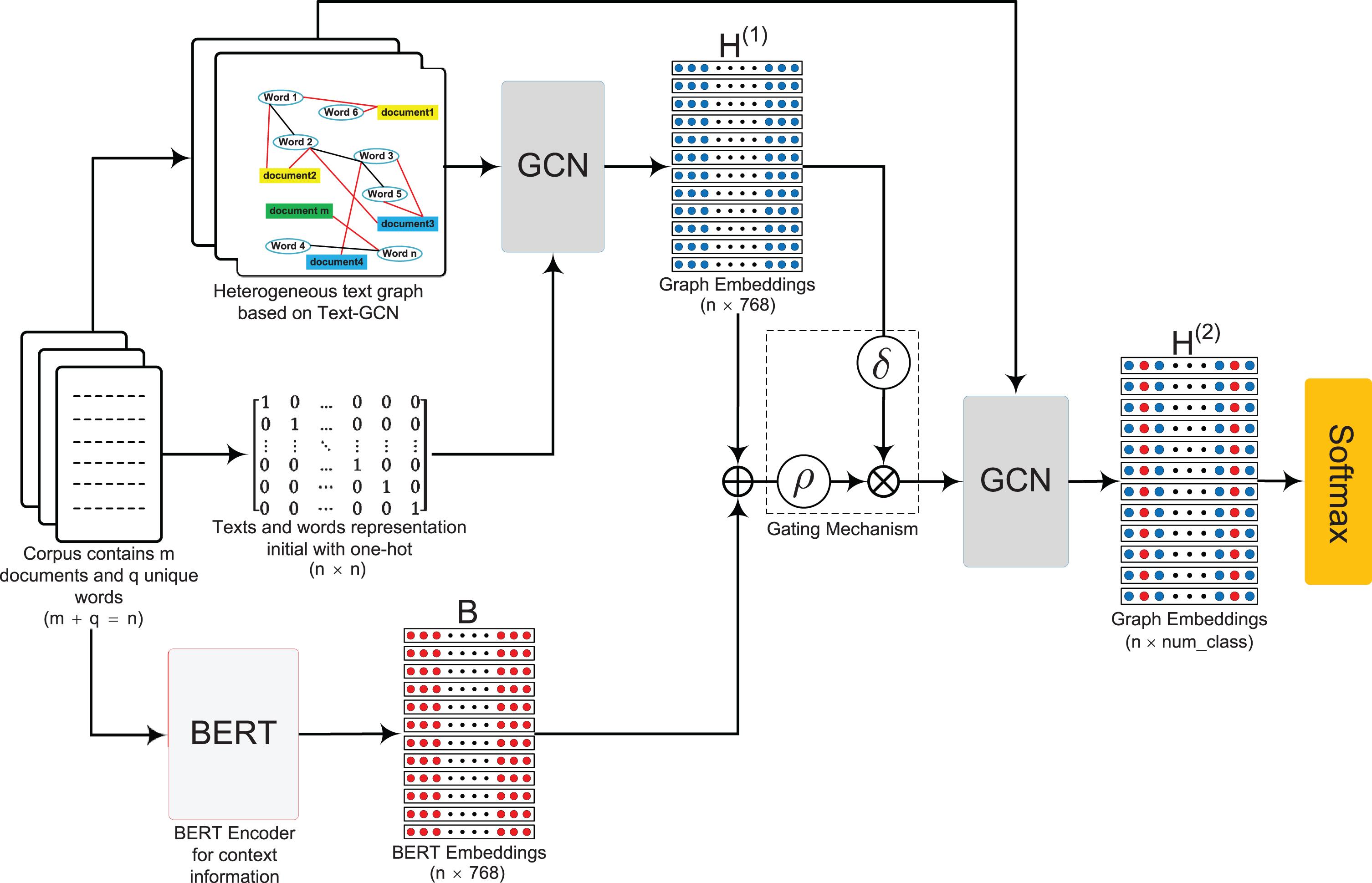
Schematic of GC-GCN. The heterogeneous text graph is based on Text-GCN [14], in which the circles represents q unique words (vocabulary size), the boxes stand for m documents (or sentences), where boxes of the same color represent those belonging to the same label, and q + m is the total number of nodes n. Red lines are document (sentence)–word edges and black lines are word–word edges. The original input feature is one-hot, $H^{(1)} \in ℝ^{n \times 768}$ is used both as input to part of the next layer and as a gating mechanism, $B \in ℝ^{n \times 768}$ is the BERT embedding, the input of second GCN layer is ρ (H⁽¹⁾ ⊕ B) ⊗ δ (H⁽¹⁾), ρ and δ are the activation functions (e.g., tanh or Sigmoid), and $H^{(2)} \in ℝ^{n \times num_class}$ is the output of the second GCN layer, which was sent to softmax for classification.

$\begin{matrix} Y = softmax (S ρ (ReLU ({SIW}^{(1)}) \oplus B) \\ \otimes δ (ReLU ({SIW}^{(1)})) W^{(2)}), \end{matrix}$ (12) where $W^{(2)} \in ℝ^{768 \times c}$ is the weight matrix of the second graph convolutional layer. We can also obtain the smoothed representation matrix $\hat{Y} \in ℝ^{n \times 768}$ by Eq. (3): $\begin{matrix} \hat{Y} \leftarrow S ρ (ReLU ({SIW}^{(1)}) \oplus B) \\ \otimes δ (ReLU ({SIW}^{(1)})) . \end{matrix}$ (13) From Eq. (4), we can intuitively see the process of feature propagation in detail: $\begin{matrix} {\hat{y}}_{i} \leftarrow \frac{1}{d_{i} + 1} ρ (h_{i}^{(1)} \oplus b_{i}) \otimes δ (h_{i}^{(1)}) + \\ \sum_{j = 1}^{n} \frac{a_{ij}}{\sqrt{(d_{i} + 1) (d_{j} + 1)}} ρ (h_{j}^{(1)} \oplus b_{j}) \otimes δ (h_{j}^{(1)}) \end{matrix},$ (14) where ${\hat{y}}_{i}$ is the smoothed feature vector (of dimension 768) for node n_i, based on its related nodes. From Eq. (13), we can directly see that ${\hat{y}}_{i}$ contains both global structural information $h_{i}^{(1)}$ and context information b_i, which somewhat overcomes the fact that Text-GCN [14] does not consider the context information in the text. Furthermore, the gating mechanism can preserve useful information in the training step [15]. Finally, like most classification tasks, Cross-entropy is applied to our model as the loss function: $L = - \sum_{d \in Y_{D}} \sum_{c = 1}^{C} {\tilde{Y}}_{dc} ln Y_{dc},$ (15) where $Y_{D}$ is the labeled document set, C is the dimension of the final output features (which is equal to the number of classes), and $\tilde{Y}$ is the label indicator matrix.

4 Experiments

In this section, we compare our proposed model to Text-GCN on multiple datasets from various aspects, such as classification accuracy, visualization of learned features and changing the size of the training set. For GC-GCN, we use GloVe word embeddings [36] (http://nlp.stanford.edu/data/glove.6B.zip) for the document representation [37] for comparison with BERT embeddings, and mathematical analysis and experimental verification of a variety of gating mechanisms with different activation functions. Finally, we use Euclidean distance to construct the text graph of the MR dataset, and compare GC-GCN with Text-GCN on the new graph data.

4.1 Datasets

To make fair comparison with Text-GCN, we used the same benchmark corpora from [14]: 20-Newsgroups (20NG), Ohsumed, R52, R8, and binary Movie Review sentiment classification data (MR). We pre-processed these corpora according to [14]. All the datasets are available online (https://github.com/yao8839836/text_gcn/tree/master/data). The overview of the datasets were shown in Table 1.

Table 1
Overview of the datasets. Sparsity describes the sparsity of data in a dataset

Datasets Docs/Sentences Training Test Vocabulary size Nodes (n) Classes Average Length (L) Sparsity

20NG 18,846 11,314 7,532 42,757 61,603 20 221.26 278

R8 7,674 5,485 2,189 7,688 15,362 8 65.72 234

R52 9,100 6,532 2,568 8,892 17,992 52 69.82 258

Ohsumed 7,400 3,357 4,043 14,157 21,557 23 135.82 159

MR 10,662 7,108 3,554 18,764 29,426 2 20.39 1443

Datasets	Docs/Sentences	Training	Test	Vocabulary size	Nodes (n)	Classes	Average Length (L)	Sparsity
20NG	18,846	11,314	7,532	42,757	61,603	20	221.26	278
R8	7,674	5,485	2,189	7,688	15,362	8	65.72	234
R52	9,100	6,532	2,568	8,892	17,992	52	69.82	258
Ohsumed	7,400	3,357	4,043	14,157	21,557	23	135.82	159
MR	10,662	7,108	3,554	18,764	29,426	2	20.39	1443

4.2 Baselines

We compared GC-GCN with several state-of-the-art text classification models. In this work, the comparisons are mainly made between GC-GCN and Text-GCN.

Text-GCN: A graph-based model for text classification proposed in [14]. It considers word-to-word mutual information and word-to-document TF–IDF information to construct a large text graph for a corpus and learns a graph embedding by GCN for text classification.

CNN: A Convolutional Neural Network-based text classification model [12], which employs convolution and the max pooling operation on word embeddings to extract features for text classification.

LSTM: The LSTM model defined in [38], which uses the last hidden state as the representation of the whole sentence for classification. Bi-LSTM is another LSTM which operates bi-directionally.

fastText: A simple and efficient method of text representation proposed in [37], which uses average word or n-gram embeddings as document embeddings and sends them into a linear classifier.

BERT+LR: Using BERT as the encoder to obtain a document representation and Logistic Regression as the classifier.

G-GCN-768: Only the gating mechanism was retained, and the context information of BERT was discarded. 768 is the number of hidden units.

C-GCN-BERT: Only the context information of BERT is retained, and no gating mechanism was used.

GC-GCN-GloVe: Word vector initialized by GloVe embedding and average them to get a document embedding, and then, applied it to GC-GCN model.

GC-GCN-Word2vec: Similar to GC-GCN-GloVe, Word vector initialized by Word2vec embedding and average them to get a document embedding, and then, applied it to GC-GCN model.

GC-GCN-GPT: GC-GCN-GPT uses pretrained model GPT [39], which also uses transformer as encoder to obtain document embeddings, and applied it to GC-GCN model.

4.3 Implementation details

We implemented our models using PyTorch-1.3.0. For GC-GCN, we set the number of hidden units in the first graph convolutional layer to 768 in accordance with the dimensions of the BERT feature vectors. As for Eq. (10), we did not set the activation functions for F and H⁽¹⁾, which will be explained in Section 4.5. We set the window size to 20 when calculating the PMI, and randomly select 10% of the training set as the validation set. In the training step, we use gradient descent with the Adam [40] update rule. The initial learning rate is 0.04, and then, drops by 20% every five steps in the first 25 steps. The maximum number of epochs was 200 and training was stopped if the validation loss did not decrease for 10 consecutive epochs.

We also tested the effect of adding layers to our model, and found that our model achieved the best results with two layers; this is because deeper GCNs can suffer from over-smoothing problems [41].

4.4 Experimental results

4.4.1 Results in existing literature

Table 2 presents the test accuracy of from the models on the five benchmark datasets. We can see the results based on Text-GCN are better than those of the other traditional neural-based models, such as CNN, LSTM, and fastText, which is likely due to the graph network structure’s ability to transmit rich adjacency information in the graph data. Meanwhile, it also leads to indirect learning of label information between different nodes. These characteristics do not exist in other deep learning methods. In this paper, we mainly focus on comparing GC-GCN against Text-GCN; from Table 2, we can see that GC-GCN-BERT achieved state-of-the-art results on the 20NG, R8, R52 and Ohsumed. As for why GC-GCN-BERT did not outperform Text-GCN on MR, we consider that in more detail.

Table 2
Test Accuracy on text classification. The results above the horizontal line in the table were taken from [14]. All models were run 10 times and report the mean ± standard deviation

Models 20NG R8 R52 Ohsumed MR

CNN-rand 76.93 ± 0.61 94.02 ± 0.57 85.37 ± 0.47 43.87 ± 0.10 74.98 ± 0.70

CNN-non-static 82.15 ± 0.52 95.71 ± 0.52 87.59 ± 0.48 58.44 ± 0.11 77.75 ± 0.72

LSTM 65.71 ± 0.15 93.68 ± 0.82 85.54 ± 0.11 41.13 ± 0.12 75.06 ± 0.44

LSTM (pretrain) 75.43 ± 0.17 96.09 ± 0.19 90.48 ± 0.86 51.10 ± 1.50 77.33 ± 0.89

Bi-LSTM 73.18 ± 0.19 96.31 ± 0.33 90.54 ± 0.91 49.27 ± 0.11 77.68 ± 0.86

fastText 79.38 ± 0.30 96.13 ± 0.21 92.81 ± 0.09 57.70 ± 0.49 75.14 ± 0.20

Text-GCN 86.34 ± 0.09 97.07 ± 0.10 93.56 ± 0.18 68.36 ± 0.56 76.74 ± 0.20

BERT+LR 73.34 ± 0.22 96.26 ± 0.28 91.49 ± 0.21 54.65 ± 0.57 81.07 ± 0.36

GloVe+LR 72.36 ± 0.13 97.02 ± 0.09 92.20 ± 0.19 55.09 ± 0.28 75.99 ± 0.52

Text-GCN-200 86.12 ± 0.08 96.90 ± 0.05 93.87 ± 0.13 68.39 ± 0.32 76.29 ± 0.24

Text-GCN-300 86.21 ± 0.16 97.09 ± 0.11 93.95 ± 0.13 68.42 ± 0.44 75.76 ± 0.38

Text-GCN-768 86.39 ± 0.12 97.14 ± 0.12 94.04 ± 0.12 68.45 ± 0.24 74.36 ± 0.61

G-GCN-768 86.28 ± 0.13 97.56 ± 0.09 94.53 ± 0.16 69.34 ± 0.22 75.82 ± 0.73

C-GCN-BERT 86.20 ± 0.17 97.26 ± 0.13 94.13 ± 0.18 67.33 ± 0.43 71.22 ± 1.29

GC-GCN-Word2vec 83.67 ± 0.12 96.77 ± 0.05 93.62 ± 0.09 63.22 ± 0.35 73.24 ± 0.31

GC-GCN-GPT 86.10 ± 0.02 96.32 ± 0.06 93.57 ± 0.03 67.22 ± 0.33 74.21 ± 0.39

GC-GCN-Glove 84.67 ± 0.20 97.23 ± 0.14 93.84 ± 0.14 64.68 ± 0.28 76.76 ± 0.11

GC-GCN-BERT 86.47 ± 0.08 97.64 ± 0.05 94.61 ± 0.14 69.53 ± 0.21 76.25 ± 0.29

Models	20NG	R8	R52	Ohsumed	MR
CNN-rand	76.93 ± 0.61	94.02 ± 0.57	85.37 ± 0.47	43.87 ± 0.10	74.98 ± 0.70
CNN-non-static	82.15 ± 0.52	95.71 ± 0.52	87.59 ± 0.48	58.44 ± 0.11	77.75 ± 0.72
LSTM	65.71 ± 0.15	93.68 ± 0.82	85.54 ± 0.11	41.13 ± 0.12	75.06 ± 0.44
LSTM (pretrain)	75.43 ± 0.17	96.09 ± 0.19	90.48 ± 0.86	51.10 ± 1.50	77.33 ± 0.89
Bi-LSTM	73.18 ± 0.19	96.31 ± 0.33	90.54 ± 0.91	49.27 ± 0.11	77.68 ± 0.86
fastText	79.38 ± 0.30	96.13 ± 0.21	92.81 ± 0.09	57.70 ± 0.49	75.14 ± 0.20
Text-GCN	86.34 ± 0.09	97.07 ± 0.10	93.56 ± 0.18	68.36 ± 0.56	76.74 ± 0.20
BERT+LR	73.34 ± 0.22	96.26 ± 0.28	91.49 ± 0.21	54.65 ± 0.57	81.07 ± 0.36
GloVe+LR	72.36 ± 0.13	97.02 ± 0.09	92.20 ± 0.19	55.09 ± 0.28	75.99 ± 0.52
Text-GCN-200	86.12 ± 0.08	96.90 ± 0.05	93.87 ± 0.13	68.39 ± 0.32	76.29 ± 0.24
Text-GCN-300	86.21 ± 0.16	97.09 ± 0.11	93.95 ± 0.13	68.42 ± 0.44	75.76 ± 0.38
Text-GCN-768	86.39 ± 0.12	97.14 ± 0.12	94.04 ± 0.12	68.45 ± 0.24	74.36 ± 0.61
G-GCN-768	86.28 ± 0.13	97.56 ± 0.09	94.53 ± 0.16	69.34 ± 0.22	75.82 ± 0.73
C-GCN-BERT	86.20 ± 0.17	97.26 ± 0.13	94.13 ± 0.18	67.33 ± 0.43	71.22 ± 1.29
GC-GCN-Word2vec	83.67 ± 0.12	96.77 ± 0.05	93.62 ± 0.09	63.22 ± 0.35	73.24 ± 0.31
GC-GCN-GPT	86.10 ± 0.02	96.32 ± 0.06	93.57 ± 0.03	67.22 ± 0.33	74.21 ± 0.39
GC-GCN-Glove	84.67 ± 0.20	97.23 ± 0.14	93.84 ± 0.14	64.68 ± 0.28	76.76 ± 0.11
GC-GCN-BERT	86.47 ± 0.08	97.64 ± 0.05	94.61 ± 0.14	69.53 ± 0.21	76.25 ± 0.29

4.4.2 Results by Text-GCN using various dimensions of first graph convolutional layer

The results of Text-GCN are taken from the original paper [14], in which Text-GCN was implemented on Tensorflow with 200 dimensions of first graph convolutional layer. In order to make a fair comparison, we designed a series of new experiments, where Text-GCN-200, Text-GCN-300, and Text-GCN-768 were implemented in PyTorch (the numbers after Text-GCN stand for the dimensions of first graph convolutional layer: 200, 300, and 768, respectievly). All the parameters of Text-GCN were set according to [14]. We conducted the significant tests between GC-GCN-BERT and Text-GCN-768 on five datasets, and the p-values are 0.042, 0.012, 0.025, 0.005 and 0.008 respectively on the 20NG, R8, R52, Ohsumed and MR dataset, indicating the significance of the improvements from the proposed GC-GCN-BERT.

From Table 2, we can see the larger the dimensions of the first graph convolutional layer of Text-GCN, the better the results on 20NG, R8, R52, and Ohsumed; while a larger dimensions of first graph convolutional layer of Text-GCN is not good for the accuracy on MR. We think that this is due to the data itself. According to Eq. (8), when we one-hot initialize the node representations, the normalized symmetric adjacency matrix $S \in ℝ^{n \times n}$ can be regarded as the representation matrix of the nodes, where n is the number of nodes and, so, the dimension of the feature vector for node n_i is n. From Table 1, we use the number of nodes n in a corpus divided by the average length L of the corpus to measure the sparsity of the corpus ( $sp = \frac{n}{L}$ ); the larger the value of sp, the more sparse the data. The sparsity of 20NG, R8, R52, Ohsumed, and MR are about 278, 234, 258, 159, and 1443, respectively. Therefore, MR is very sparse, compared to the other datasets. This led to a decrease in accuracy of Text-GCN model on MR when the dimensions of first graph convolutional layer increased. There is another reason for the decline in the MR result: the adjacency matrix was constructed using PMI and TF–IDF and the sentences in the MR are very short and, so, PMI and TF–IDF were not suitable for building the adjacency matrix in this case.

4.4.3 Results by gating mechanism or context information

From G-GCN-768, we see the gating mechanism can effectively improve the classification accuracy on R8, R52, Ohsumed and MR compared with Text-GCN-768. In C-GCN-BERT, directly adding context information into the graph embedding can only get a slight improvement on R8 and R52, and even significantly decrease on 20NG, Ohsumed and MR compared with Text-GCN-768. As for the GC-GCN-BERT model, we find that GC-GCN-BERT combined the merits of the gating mechanism and BERT to boost its performance.

4.4.4 Results by different document representations

From Table 2, we can see that BERT+LR performs the best on the MR. From the above discussion we have learnt that MR is a short text dataset for binary sentiment classification, and contextual information is very important in the task of sentiment classification. Given BERT’s excellent performance on the MR, we know that BERT takes good account of the context information of words when encoding text. GloVe+LR achieves better results than BERT+LR on R8, R52, and Ohsumed, but does not outperform BERT+LR on MR; this is because, in the sentiment classification problem, the BERT encoder considers the context information in the text, which the document representation of GloVe embedding does not.

Text-GCN-300 is a comparison experiment of GC-GCN-GloVe, as the first convolutional layer of the two models all had dimension 300. The accuracy of GC-GCN-GloVe was about 1% higher than Text-GCN-300 on MR; GC-GCN-BERT obtained a relative poor result on MR, due to the sparsity of the data, but the gain of GC-GCN-BERT over Text-GCN-768 was about 1.89%, which greater than that of GC-GCN-GloVe over Text-GCN-300. We can also see that the accuracy of GC-GCN-GloVe on 20ng and Ohsumed were worse than those of GC-GCN-300; we also used Word2vec based embedding and the pretrained model GPT in GC-GCN, the results of GC-GCN-Word2vec and GC-GCN-GPT were poor, so the Word2vec based embeddings and GPT based embedding do not apply to GC-GCN; these suggest that, when we apply GC-GCN model, we need to select an appropriate context embedding.

4.4.5 Results by combine gating mechanism and context information

GC-GCN after choosing an appropriate document representation BERT, GC-GCN-BERT obtained the best results on four out of five datasets in Table 2. This is because the gating mechanism integrates the context information with graph embedding so that GC-GCN-BERT has the ability to process context information which is not available in Text-GCN. We can find that GC-GCN-BERT can mitigate the problem of sparse data on MR, making the result of GC-GCN-BERT on MR is close to that of Text-GCN-200.

4.5 Analysis of gating mechanism

Table 3 shows the accuracy of GC-GCN-BERT in R8, R52 and Ohsumed by using the gating mechanisms with different activation functions. Inspired by [15], we used different activation functions to verify the gating mechanism. By Eq. (10), we can define the gradient of the Gated Tanh Unit (GTU), where the activation function of F is tanh, as follows: $\begin{matrix} \nabla [tanh (F) \otimes δ (H^{(1)}] = {tanh}^{'} (F) \nabla F \\ \otimes δ (H^{(1)}) \oplus δ^{'} (H^{(1)} \nabla H^{(1)} \otimes tanh (F)), \end{matrix}$ (16) where δ is an activation function such as ReLU or Sigmoid. This is more likely to cause the vanishing gradient problem, due to the presence of the downscaling factors [15] tanh ′ (F) and δ′ (H⁽¹⁾. There is another gating mechanism, called a Gated Linear Unit (GLU), in which the activation function of F is removed. The gradient of a GLU is $\begin{matrix} \nabla [F \otimes δ (H^{(1)})] = \nabla F \otimes δ (H^{(1)} \\ \oplus F \otimes δ^{'} (H^{(1)} \nabla H^{(1)})) . \end{matrix}$ (17)

Table 3

The accuracy of different activation mechanisms on the datasets R8, R52, and Ohsumed.

Sigmoid, Tanh, and ReLU are the different activation functions of the GLU. We tested all models 10 times and report the mean ± standard deviation

Gating Mechanism	R8	R52	Ohsumed
GTU	97.01 ± 0.08	93.83 ± 0.16	68.68 ± 0.16
GLU-Sigmoid	97.34 ± 0.08	94.25 ± 0.13	69.26 ± 0.18
GLU-Tanh	97.56± 0.08	94.33± 0.09	69.31± 0.09
GLU-ReLU	97.69± 0.08	94.59± 0.09	69.45± 0.14
Text-GCN-768	97.14 ± 0.12	94.04 ± 0.12	68.45 ± 0.24
Bi-GLU	97.64± 0.05	94.61± 0.14	69.53± 0.21

We can see that ∇F ⊗ δ (H⁽¹⁾ does not have a downscaling factor and, so, it suffers from less gradient vanishing than in the GTU. In a Bi-directional Gated Linear Unit (Bi-GLU), both the activation functions of F and H⁽¹⁾ are removed; we obtain the gradient of a Bi-GLU as $\nabla [F \otimes H^{(1)}] = \nabla F \otimes H^{(1)} \oplus F \otimes \nabla H^{(1)} .$ (18) We can observe that using a Bi-GLU is a good way to address the vanishing gradient problem of GTU and GLU, due to there being no downscaling factor in gradient propagation.

From Table 3, GTU with the Sigmoid activation function demonstrates poor results, due to the vanishing gradient problem. The different activation function used in the gated linear unit (GLU) achieves better results than Text-GCN-768. Bi-GLU obtained the best results on R52 and Ohsumed, and the gated linear unit with the ReLU activation function (GLU-ReLU) achieved best result on R8, it was about 0.55%, 0.55% and 1% higher than Text-GCN-768 in datasets R8, R52 and Ohsumed. Actually, the GLU with the ReLU activation function and Bi-GLU are gated linear units of the same type and, so, their results were similar. However, Bi-GLU has a higher computational efficiency than the former, as it does not have to compute the derivative of ReLU during gradient propagation. Therefore, we found Bi-GLU to be suitable for our model.

4.6 Visualization

Figure 3 and Figure 4 use t-SNE tool [42] to show the Visual distribution of first and second layer embeddings learnt by Text-GCN-768, C-GCN-BERT and GC-GCN-BERT in the test set of R8 respectively. From Figure 3, We can intuitively see that GC-GCN-BERT and C-GCN-BERT had better clustering ability than Text-GCN-768, and that GC-GCN-BERT achieved the best performance. Figure 4 shows the Visual distribution of second layer embeddings in the test set of R8. It can be found that the document representation of each category learnt by GC-GCN-BERT is more effective than the clustering of Text-GCN-768 and C-GCN-BERT, especially the clustering of aca and earn, so GC-GCN-BERT achieved the best results in terms of classification accuracy. Secondly, the classification accuracy of C-GCN-BERT is higher than that of Text-GCN-768, so we can see that C-GCN-BERT was better than Text-GCN-768 at distinguishing between the classes "crude", "acq", and "trade".

Fig. 3

The t-SNE visualization of test set document embeddings of the first layer learnt by Text-GCN-768, C-GCN-BERT, and GC-GCN-BERT in R8.

Fig. 4

The t-SNE visualization of test set document embeddings of the second layer learnt by Text-GCN-768, C-GCN-BERT, and GC-GCN-BERT in R8.

4.7 Analysis of the size of labeled data

Figure 5 shows the test accuracy when using 1%, 5%, 10%, and 20% of the original R8 and 20NG training sets. We can see that GC-GCN-BERT was better and more stable than Text-GCN-768, except for when the proportion of training set on 20NG was 1%; this was mainly related to the number of classes in the dataset. R8 had 8 classes and 20NG had 20 classes. When the training set was scaled down, for the dataset with a large number of classes, some classes may be eliminated from the training set altogether, which is more likely to happen than in datasets with a relatively small number of classes. Text-GCN-768 uses global word co-occurrence and TF–IDF information to generate the graph embedding but, in the case of GC-GCN-BERT, the learned graph embeddings add context information, so that the document representation learnt by GC-GCN-BERT is more targeted. Therefore, when the training set is scaled down significantly, GC-GCN-BERT cannot learn all the class information of a dataset with a large number of classes completely, as the information of the current text is added by BERT features, and as some classes may have been removed before training; therefore, the accuracy of the GC-GCN-BERT results may decrease significantly. However, for datasets with a small number of classes, GC-GCN-BERT is still better than Text-GCN when the training set is reduced significantly.

Fig. 5

Test accuracy when altering the size of the training set. We used Text-GCN-768 and GC-GCN-BERT to test 10 times on R8 and 20NG, and report the mean ± standard deviation.

4.8 Incorporating Euclidean distance into MR text graph

As has been discussed above, PMI or TF–IDF information alone is not sufficient to build a text graph on MR. So in this section, we use the Euclidean distance to build the adjacency matrix for the MR, in order to evaluate the influence of the adjacency matrix. It is found that a learning rate of 0.03 for our model is better for the new data. We directly use the BERT features to calculate the word–word E_ww and word–document E_wd Euclidean distances, due to its excellent performance in sentiment classification. Then, we set the PMI and TF–IDF values to W_p and W_t, respectively, and set α as the weight to calculate the new word–word and word–document information, where the new word–word information was α × E_ww + (1 - α) × W_p and the new word–document information was α × E_wd + (1 - α) × W_t.

Table 4 and Figure 6 show the accuracy of the GC-GCN and Text-GCN models when using different weights α. Text-GCN-200 and Text-GCN-768 denote that the hidden dimensions of first graph convolutional layer used in Text-GCN were 200 and 768 respectively, and their learning rate was set to 0.02, according to [14]. GC-GCN-CLR adopted the changing learning rate rule, GC-GCN-0.03 had a fixed learning rate of 0.03, and the context information used by GC-GCN was the BERT features. We can see that, when the value of α was set at 0.5 and 1, GC-GCN and Text-GCN achieved their best results, respectively. We note that, when the value of α was small (in other words, when the proportion of PMI and TF–IDF was large), the results of Text-GCN were relatively poor, This means that PMI and TF–IDF were not suitable for constructing an adjacency matrix for the MR. After incorporating Euclidean distance weighting, the accuracy of GC-GCN-0.03 was about 0.28% higher than LSTM (pre-trained) and very close to the result of Bi-LSTM, which handles context information well; this indicates that GC-GCN also has the ability to handle context information.

Table 4
The accuracy after combining Euclidean distance with PMI and TF–IDF, using different weights α on the MR. We tested these new data on the GC-GCN-BERT and Text-GCN models 10 times repectively, and report the mean ± standard deviation

α Text-GCN-200 Text-GCN-768 GC-GCN-CLR GC-GCN-0.03

0 76.23 ± 0.24 74.32 ± 0.52 76.25±0.29 76.11 ± 0.48

0.1 76.55±0.27 74.32 ± 0.52 76.58±0.52 76.24 ± 0.16

0.2 76.70± 0.32 74.30 ± 0.79 77.03±0.59 76.45 ± 0.31

0.3 76.66 ±0.22 74.53± 0.84 77.11±0.34 77.17± 0.08

0.4 76.77±0.31 74.32± 0.50 76.96±0.43 77.38± 0.30

0.5 76.86±0.33 74.69 ± 1.11 77.19±0.43 77.61 ± 0.21

0.6 76.87±0.39 74.81± 0.60 76.84±0.35 77.47± 0.22

0.7 77.03±0.40 74.74± 0.58 76.95±0.35 77.39± 0.13

0.8 76.83±0.39 75.58± 0.67 76.69±0.55 77.20± 0.18

0.9 76.95±0.27 75.09± 0.94 76.70±0.50 77.13± 0.15

1 77.10±0.27 75.16± 0.12 76.74±0.46 77.17± 0.36

α	Text-GCN-200	Text-GCN-768	GC-GCN-CLR	GC-GCN-0.03
0	76.23 ± 0.24	74.32 ± 0.52	76.25±0.29	76.11 ± 0.48
0.1	76.55±0.27	74.32 ± 0.52	76.58±0.52	76.24 ± 0.16
0.2	76.70± 0.32	74.30 ± 0.79	77.03±0.59	76.45 ± 0.31
0.3	76.66 ±0.22	74.53± 0.84	77.11±0.34	77.17± 0.08
0.4	76.77±0.31	74.32± 0.50	76.96±0.43	77.38± 0.30
0.5	76.86±0.33	74.69 ± 1.11	77.19±0.43	77.61 ± 0.21
0.6	76.87±0.39	74.81± 0.60	76.84±0.35	77.47± 0.22
0.7	77.03±0.40	74.74± 0.58	76.95±0.35	77.39± 0.13
0.8	76.83±0.39	75.58± 0.67	76.69±0.55	77.20± 0.18
0.9	76.95±0.27	75.09± 0.94	76.70±0.50	77.13± 0.15
1	77.10±0.27	75.16± 0.12	76.74±0.46	77.17± 0.36

Fig. 6

The accuracy after combining Euclidean distance with PMI and TF–IDF, using different weights α on the MR.

5 Conclusions and future work

In this paper, we have proposed a simple and effective model for text classification named as GC-GCN. We use the graph convolutional network as a gating mechanism to integrate BERT’s context information with graph embedding, thus overcoming the problem of not considering context information in Text-GCN. We compared GC-GCN and Text-GCN on multiple datasets in terms of classification accuracy, visualization of learned features, and the accuracy of changing the size of the training set, and found that GC-GCN performed better than Text-GCN. Especially in classification accuracy, The GC-GCN has respectively obtained 0.19%, 0.57%, 1.05% and 1.17% improvements over the Text-GCN baseline on the 20NG, R8, R52, and Ohsumed benchmark datasets. We also used different document representations to illustrate BERT embedding’s suitability for GC-GCN. Further more, we used the Euclidean distance in a weighted sum with PMI and TF–IDF when constructing the adjacency matrix to address the problem that PMI and TF–IDF are not suitable for short data (i.e., the MR), and it was about 1.38% higher than Text-GCN on MR. In future research, we will consider the fine-tuning of the BERT Encoder during the GC-GCN training step, which can provide more precise context information for the current corpus.

Footnotes

Acknowledgments

This work is funded by National Key R&D Program of China (2017YFB1402101); Natural Science Foundation of China (61663044); Opening Project of Key Laboratory of Xinjiang Uyghur Autonomous Region, China.

References

Pang

, Lee

, others, Opinion mining and sentiment analysis, Foundations and Trends® in Information Retrieval 2 (2008), 1–135.

Aggarwal

C.C.

and Zhai

, A survey of text classification algorithms. In Mining text data; Springer, 2012; pp. 163–222.

Zeng

, Deng

, Li

, Naumann

and Luo

, Natural language processing for EHR-based computational phenotyping, IEEE/ACM transactions on computational biology and bioinformatics 16 (2018), 139–153.

Cer

, Yang

, Kong

, Hua

, Limtiaco

, John

R.S.

, Constant

, Guajardo-Cespedes

, Yuan

, Tar

, Sung

, Strope

and Kurzweil

, Universal Sentence Encoder, CoRR (2018), abs/1803.11175.

Zelikovitz

and Hirsh

, Using LSI for text classification in the presence of background text, Proceedings of the tenth international conference on Information and knowledge management, ACM, 2001, pp. 113–118.

Joachims

, Text categorization with support vector machines: Learning with many relevant features, European conference on machine learning. Springer, 1998, pp. 137–142.

Cavnar

W.B.

, Trenkle

J.M.

, others, N-gram-based text categorization, Proceedings of SDAIR-94, 3rd annual symposium on document analysis and information retrieval, Citeseer, 1994, Vol. 161175.

Chandrasekaran

, Periyasamy

and Karthikeyan

P.R.

, Test scheduling for system on chip using modified firefly and modified abc algorithms, SN Applied Sciences 1(9) (2019), 1079.

Chandrasekaran

, Periyasamy

and Karthikeyan

P.R.

, Minimization of test time in system on chip using artificial intelligence-based test scheduling techniques, Neural Computing and Applications, pages 1–10, 2019.

10.

LeCun

, Bengio

and Hinton

, Deep learning, nature 521 (2015), 436–444.

11.

Hochreiter

and Schmidhuber

, Long Short-Term Memory, Neural Computation 9 (1997), 1735–1780.

12.

Kim

, Convolutional Neural Networks for Sentence Classification, Proceedings of the 2014 Conference on Empirical Methods in Natural Language Processing (EMNLP); Association for Computational Linguistics: Doha, Qatar, 2014; pp. 1746–1751.

13.

Kipf

T.N.

and Welling

, Semi-Supervised Classification with Graph Convolutional Networks, International Conference on Learning Representations (ICLR), 2017.

14.

Yao

, Mao

and Luo

, Graph convolutional networks for text classification, , Proceedings of the AAAI Conference on Artificial Intelligence 33 (2019), 7370–7377.

15.

Dauphin

Y.N.

, Fan

, Auli

and Grangier

, Language modeling with gated convolutional networks, Proceedings of the 34th International Conference on Machine Learning- Volume 70. JMLR. org, 2017, pp. 933–941.

16.

Zhang

, Jin

and Zhou

Z.H.

, Understanding bag-of-words model: a statistical framework, International Journal of Machine Learning and Cybernetics 1 (2010), 43–52.

17.

Blei

D.M.

, Ng

A.Y.

and Jordan

M.I.

, Latent dirichlet allocation, Journal of Machine Learning Research 3 (2003), 993–1022.

18.

Rish

, others, An empirical study of the naive Bayes classifier, IJCAI 2001 workshop on empirical methods in artificial intelligence, 2001, Vol. 3, pp. 41–46.

19.

Tong

and Koller

, Support vector machine active learning with applications to text classification, Journal of machine learning research 2 (2001), 45–66.

20.

Bengio

, Ducharme

, Vincent

and Jauvin

, A neural probabilistic language model, Journal of machine learning research 3 (2003), 1137–1155.

21.

Hinton

G.E.

, others, Learning distributed representations of concepts, Proceedings of the eighth annual conference of the cognitive science society, Amherst, MA, 1986, Vol. 1, p. 12.

22.

Mikolov

, Chen

, Corrado

and Dean

, Efficient estimation of word representations in vector space, Computer Science (2013).

23.

Mikolov

, Sutskever

, Chen

, Corrado

G.S.

and Dean

, Distributed representations of words and phrases and their compositionality, Advances in neural information processing systems, 2013, pp. 3111–3119.

24.

Socher

, Huang

E.H.

, Pennin

, Manning

C.D.

and Ng

A.Y.

, Dynamic pooling and unfolding recursive autoencoders for paraphrase detection, Advances in neural information processing systems, 2011, pp. 801–809.

25.

Devlin

, Chang

M.W.

, Lee

and Toutanova

, BERT: Pre-training of Deep Bidirectional Transformers for Language Understanding, Proceedings of the 2019 Conference of the North American Chapter of the Association for Computational Linguistics: Human Language Technologies, Volume 1 (Long and Short Papers), 2019, pp. 4171–4186.

26.

Vaswani

, Shazeer

, Parmar

, Uszkoreit

, Jones

, Gomez

A.N.

, Kaiser

Ł.

and Polosukhin

, Attention is all you need, Advances in neural information processing systems, 2017, pp. 5998–6008.

27.

Peters

M.E.

, Neumann

, Iyyer

, Gardner

, Clark

, Lee

and Zettlemoyer

, Deep contextualized word representations, Proceedings of NAACL-HLT, 2018, pp. 2227–2237.

28.

Sorokin

, and I, Gurevych, Modeling Semantics with Gated Graph Neural Networks for Knowledge Base Question Answering, Proceedings of the 27th International Conference on Computational Linguistics, 2018, pp. 3306–3317.

29.

Marcheggiani

and Titov

, Encoding Sentences with Graph Convolutional Networks for Semantic Role Labeling, Proceedings of the 2017 Conference on Empirical Methods in Natural Language Processing; Association for Computational Linguistics: Copenhagen, Denmark, 2017; pp. 1506–1515.

30.

Bastings

, Titov

, Aziz

, Marcheggiani

and Sima’an

, Graph Convolutional Encoders for Syntax-aware Neural Machine Translation, Proceedings of the 2017 Conference on Empirical Methods in Natural Language Processing, 2017, pp. 1957–1967.

31.

T.J.

, Li

P.H.

and Ma

W.Y.

, GraphRel: Modeling text as graphs for joint entity and relation extraction, Proceedings of the 57th Annual Meeting of the Association for Computational Linguistics, 2019, pp. 1409–1418.

32.

Velickovic

, Cucurull

, Casanova

, Romero

, Lio

and Bengio

, Graph attention networks, stat 1050 (2018), 4.

33.

Thekumparampil

K.K.

, Wang

, Oh

and Li

L.J.

, Attention-based graph neural network for semi-supervised learning, Sixth International Conference on Learning Representations, 2018.

34.

Busbridge

, Sherburn

, Cavallo

and Hammerla

N.Y.

, Relational Graph Attention Networks, arXiv preprint arXiv:1904.05811 (2019).

35.

, Souza

, Zhang

, Fifty

, Yu

and Weinberger

, Simplifying Graph Convolutional Networks, International Conference on Machine Learning, 2019, pp. 6861–6871.

36.

Pennington

, Socher

and Manning

C.D.

, Glove: Global vectors for word representation, Proceedings of the 2014 conference on empirical methods in natural language processing (EMNLP), 2014, pp. 1532–1543.

37.

Joulin

, Grave

, Bojanowski

and Mikolov

, Bag of Tricks for Efficient Text Classification, Proceedings of the 15th Conference of the European Chapter of the Association for Computational Linguistics: Volume 2, Short Papers; Association for Computational Linguistics:Valencia, Spain, 2017; pp. 427–431.

38.

Liu

, Qiu

and Huang

, Recurrent neural network for text classification with multi-task learning, Proceedings of the Twenty-Fifth International Joint Conference on Artificial Intelligence. AAAI Press, 2016, pp. 2873–2879.

39.

Radford

, Narasimhan

, Salimans

and Sutskever

, Improving language understanding by generative pretraining.

40.

Kingma

D.P.

and Ba

, Adam: A Method for Stochastic Optimization, Computer Science (2014).

41.

, Han

and Wu

X.M.

, Deeper Insights into Graph Convolutional Networks for Semi-Supervised Learning, Proceedings of the Thirty-Second AAAI Conference on Artificial Intelligence (AAAI-18). Association for the Advancement of Artificial Intelligence, 2018, pp. 3538–3545.

42.

Maaten

L.V.D.

and Hinton

, Visualizing data using t-SNE, Journal of Machine Learning Research 9 (2008), 2579–2605.