Deep learning based algorithm (ConvLSTM) for Copy Move Forgery Detection

Abstract

Protecting information from manipulation is important challenge in current days. Digital images are one of the most popular information representation. Images could be used in several fields such as military, social media, security purposes, intelligence fields, evidences in courts, and newspapers. Digital image forgeries mean adding unusual patterns to the original images that cause a heterogeneity manner in form of image properties. Copy move forgery is one of the hardest types of image forgeries to be detected. It is happened by duplicating part or section of the image then adding again in the image itself but in another location. Forgery detection algorithms are used in image security when the original content is not available. This paper illustrates a new approach for Copy Move Forgery Detection (CMFD) built basically on deep learning. The proposed model is depending on applying (Convolution Neural Network) CNN in addition to Convolutional Long Short-Term Memory (CovLSTM) networks. This method extracts image features by a sequence number of Convolutions (CNVs) layers, ConvLSTM layers, and pooling layers then matching features and detecting copy move forgery. This model had been applied to four aboveboard available databases: MICC-F220, MICC-F2000, MICC-F600, and SATs-130. Moreover, datasets have been combined to build new datasets for all purposes of generalization testing and coping with an over-fitting problem. In addition, the results of applying ConvLSTM model only have been added to show the differences in performance between using hybrid ConvLSTM and CNN compared with using CNN only.

The proposed algorithm, when using number of epoch’s equal 100, gives high accuracy reached to 100% for some datasets with lowest Testing Time (TT) time nearly 1 second for some datasets when compared with the different previous algorithms.

Keywords

Convolutional Long Short-Term Memory (CovLSTM)copy-move forgery detection image authentication tampered images deep learning and convolutional neural networks

1 Introduction

Nowadays is known as the era of technology and information domination. At dealing with the information, there are several important challenges such as how to protect this information from manipulation and discover the executor of that attack. The most popular and wider form of the information represents in images and videos. Images are used in several sides like military purposes, social media, image recognition in security purposes, intelligence fields, evidences in courts, newspapers, defamation of public figures, and media misinformation. Because of image spread importance in community of information technology, image authentication becomes one of the important demands of information security.

The image authentication techniques are divided into two sorts; active authentication and passive authentication [1]. First, active authentication techniques are applied on the original image before using it, next the resulted image is compared with the suspected images. Active authentication techniques represented by digital signature and digital watermarking [2]. Furthermore, when the main content of the image is unobtainable, passive authentication techniques will be applied to ensure image authenticity [3]. The main differences between active and passive authentication is the previous knowledge of the original image content to examine the suspected image.

Digital image forgeries mean adding unusual patterns to the original images that cause a heterogeneity manner in form of image properties and unusual distributing of image features. Digital image forgeries are appeared in different forms like copy move forgery and other morphological application on images such as splicing, retouching, resampling, and morphing in addition to images created by graphical applications [5]. Figure 1 gives the several kinds of digital image forgeries.

Copy move forgery is utilized by taking a section or object in an image and adding it again in the image itself but in another location to conceal or iterate a specific scene in the image [3].

Splicing forgery is used by adding or merging two images or groups of images to produce an unprecedented image [6].

Retouching forgery is the process of enhancing an image to conceal or exhibit specific features like illumination, coloration, contrast enhancement, and background coloring altering [7].

Resampling Forgery is based on changing the dimensionality of a specific part or object in the image to display it in deceptive view [8].

Morphing forgery is the process of combining two various scenes of two various images to create an unprecedented scene [9].

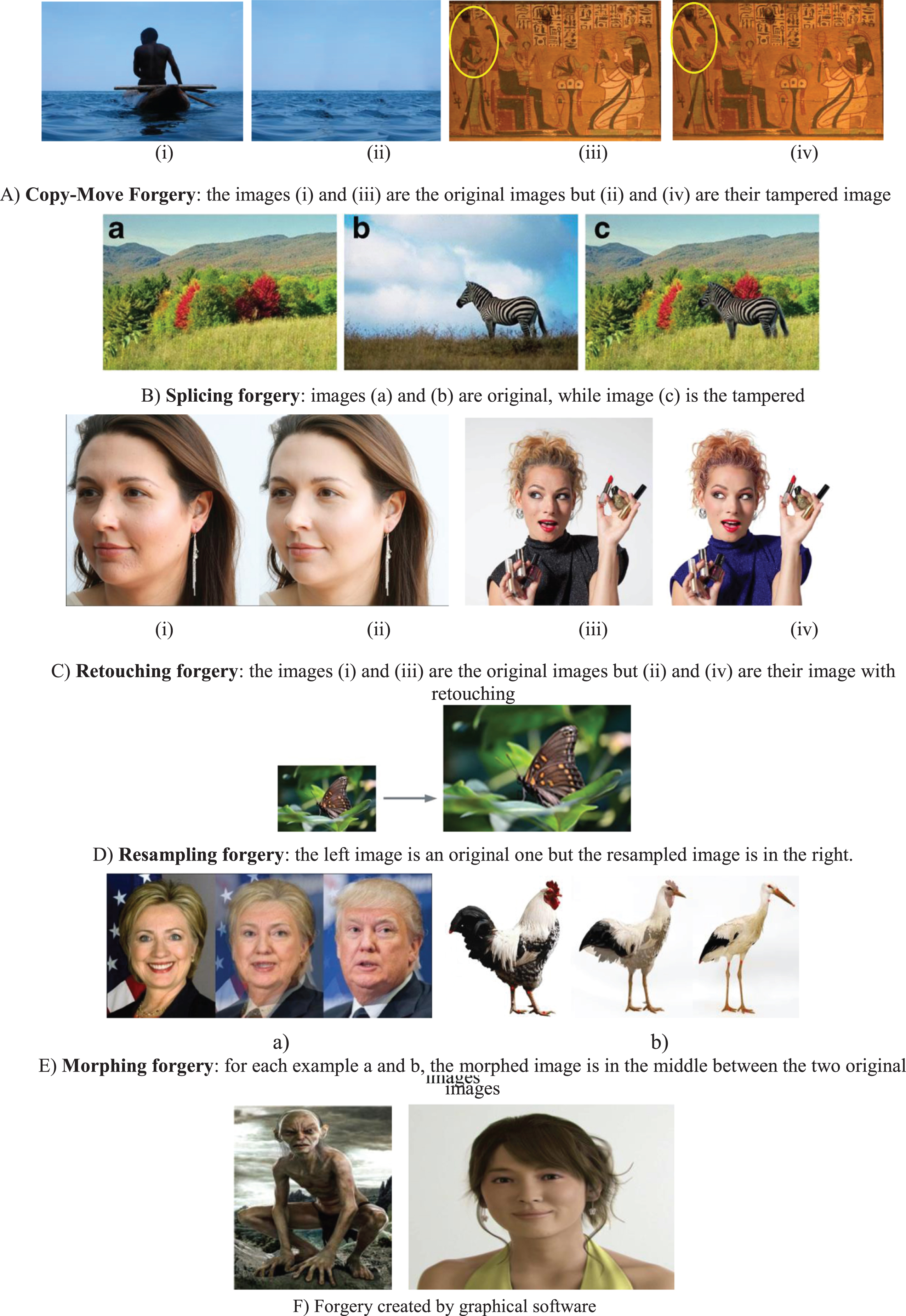
Finally, the last forgery type is applied by creating a totally image by using graphical software and the produced image is not belongs to the reality [3].

Fig.1

Several kinds for digital image forgeries.

Copy move forgery is the widest expansion forgery sort among all digital image forgeries and also it is the most difficult type to detect. As shown in the examples in Fig. 1, copy move forgery difficulty presented in copying an object or part of the image with the same properties and same features distributions and pasting it in the same image. The patched region or regions have the same properties and same features of the whole image. This method of image forgery makes the final tampered image has the same homogenous context. The final tampered image not have distortions, noise, or heterogeneity features like coloring changing, shadows, edging or any other features used as evidence of tampering.

The techniques of forgery detection are considered as one of main challenges in image security which are used with passive authentication when the premier content is unobtainable. This process depends on analyzing image features and searching for any unusual patterns [4].

This paper illustrates a new algorithm for Copy Move Forgery Detection (CMFD). This technique had proved its robustness, easy, efficiency, and speed in discovering the copy move forgery. The proposed model depends on utilizing (Convolution Neural Network) CNN in addition to Convolutional Long Short-Term Memory (CovLSTM) networks. This method extracts image features by a sequence number of Convolutions (CNVs) layers, ConvLSTM layers, and pooling layers then matching features and detecting copy move forgery.

The proposed algorithm contribution is summarized as followings:

Building a robust, easy, efficient, and fast CMFD algorithm to discover copy move forgery in digital image.

Using deep learning technique to build the proposed algorithm that automatically detected copy move forgery and extract the added features.

Increasing the detection accuracy by increasing the truly detected forgery images and decreasing the misclassified images.

The paper structure is arranged as followings. Section 2 illustrates the related work. A representation of the proposed technique will be illustrated with details in section 3. Section 4 displays detailed experimental results of the proposed algorithm which obtained by applying the proposed model on the various databases with several kinds and different difficulty levels of attacks. Section 5 gives the conclusion of the paper. Finally, the paper ends with the direction of the future work and references.

2 Related work

Digital image forensics are belonging to the science of blind or passive investigation techniques. The main challenge that faces digital image forensic algorithms is its ability to work with no preceding familiarity about the basic content of the suspected image. In the current decade, the CMFD algorithms have been categorized into traditional algorithms and deep learning based algorithms [10]. Classical models are these approaches which depends on the statistical analysis and geometrical features representations in the suspected image besides image context homogeneity [11]. The models which depends on deep learning are automatically building a classifying technique using a deep learning hypothesis such as Neural Networks (NN), Support Vector Machines (SVMs), or any other hypothesis which depends on two stages learning and testing. In learning stage, the deep learning algorithm applying image features fitting, features analyzing, and building model behavior. Furthermore, in testing stage the deep learning algorithm is automatically utilizing the building model to classify the suspected image according to complex statistical dependencies [12].

Traditional CMFD algorithms have been categorized by block-based or non-block-based techniques. Block-based techniques divided any image into blocks with different shapes varied from algorithm to another such as rectangular, overlapping, or circular blocks [13]. After division, different techniques used to extract features from each block, which acts as an image block classifier. There are many features extraction techniques, such as those that depend on frequency transformations including Discrete Cosine Transform (DCT), Discrete Wavelet Transform (DWT), Principal Component Analysis (PCA), Singular Value Decomposition (SVD), and direct fuzzy transform with ring projection [14]. In addition to the previous techniques, invariant image moments and texture and intensity descriptors techniques are also used for block-based algorithm features extraction [3]. In the final stage, the matching step is used to match similar regions or objects in the image itself according to block features matching [15].

The first use of DCT technique in CMFD is performed by Fridrich et al. [16] where the image, at the beginning, splitted to interfered blocks, after that the DCT transform had been applied on each block. Finally, image features had been represented by the extracted DCT coefficient. These coefficients are represented by a lexicographic chart for discovering the matching between the identical blocks. There are similar algorithms which extracts DCT coefficient for each block after block division operation then searching for block matching such as Maind et al. [17]. Furthermore, other algorithms are using hybrid methods to obtain higher robustness against image processing attacks like noise adding, image blurring, and image intensity changes as applied by Sunil et al. [18]. The authors in [18] are applied a combination of PCA and DCT to decrease the dimensionality of the feature vector by using low frequency DCT coefficients. Algorithm in [19] using the idea of clustering by K-means technique. This algorithm divides the image into (8 x 8) overlapping blocks after converting it from colored image into gray scale image. After that, DCT will be used on all blocks for discovering features and then clustering blocks using k-means algorithm. The final step involves a radix sorting for blocks features to perform similarity matching.

Invariant image moments techniques are used in CMFD by producing features or moments that distinguish by its stability against scaling, rotation, translation, in addition to its capability to discover location. Image moments application is like image segmentation that analyzes image objects, object orientation, detects central points, shape analysis, and regions recognition [20]. Ryu et al. [21] are using Zernike moments to discover the copy move forgery. Firstly, the algorithm converted the image to gray scale image then divided it into (a x a) overlapping blocks. Secondly, extracts Zernike moments for each block which represents the feature vectors for local image characteristics. By using Locality Sensitive Hashing (LSH) technique, a matching step will be done for discovering the copy move forgery. Reddy et al. [22] are utilizing algorithm that performs combination of Hu’s moments and DCT to CMFD. The model divided each suspected image to interfered blocks, after that rescaling this block with range from 0% to 500% in steps in which 10% in each step. In each scaling step, the corner pixels and rescale factors are sorted as feature vector. Based on comparing the matching between the sorted corner points and recalling factors obtained in each step the algorithm detects similarity or non-similarity between blocks.

Moreover, texture and intensity-based algorithms had been well performed to elicit image features and reveal copy move forgery. Analyzing of the image structure gives a huge evidence about if the image is tempered or not. The structure of the image inferred from image statistics such as pixels intensity, color changes, edges, corners, and special arrangement of color [3]. Texture and intensity-based algorithms deploying previous texture descriptors to discover the copy move forgery where, the tampering methods harms the texture and intensity arrangements of image patterns [23]. Algorithm in [24] uses mean variance to exploit statistical features of the suspected image. The image is splitted to blocks then mean variance is used as evidence about individual block with respect to image pixels intensity. Also, variance is used to show the variation between each pixel and its neighbors.

On the other side, CMFD algorithms that categorized as non-block based algorithms are called also pixel based algorithms which elicit features of each complete image [25]. Keypoints-based algorithms are the basic type of non-block based technique. these techniques depend upon keypoint descriptors in CMFD and these descriptors produce mainly from Scale Invariant Feature Transform (SIFT) and Speed Up Robust Features (SURF) [26]. David G. Lowe [27] is developed the SIFT algorithm which depends on extracting distinctive invariant features from the complete image. The most effective property of these features its invariant against scaling, translation, rotation, illumination changes, and other traditional image post-processing attacks such as blurring, noise adding, color changes, JPEG compression and affine transformation. To enhance SIFT algorithm, a fast and robust SURF algorithm is developed which produce SURF descriptors with 64 bytes size compared to 128 bytes dimensional descriptor of SIFT features [28].

Amerini et al. [29] developed a model which at the beginning discovers SIFT features of each suspected image then this image will be clustered to collect the similar features. Next, according to dynamic threshold (Euclidian distance) the similar features in different locations is detected that presents each copy move forgery parts. Algorithm at [30] utilizing the method which combines SIFT features, SURF features, and Histogram Oriented Gradient (HOG) features. Its results show that using SIFT-HOG features and SURF-HOG features produce better CMFD accuracy than using these features alone. Alberry et al. [31] proposed algorithm that used the SIFT algorithm to extracts the SIFT features then applying Fuzzy C-means (FCM) for clustering that features and searching for matching. Park et al. [32] proposed another algorithm that utilizing SIFT features and LBP histogram. At the center of each SIFT keypoint a local window is framed and the LBP values with 256 levels is obtained then reduced to only 10 levels. Finally, a similarity search is performed among LBP levels.

Recently, machine learning is used widely in different fields. One of machine learning structures is deep learning techniques that automatically used to solve many problems. CNN is one of machine learning hypothesis which used for image processing applications such as face detections in image and video, scene labelling, action recognition, image classification, and many other computer vision applications [33]. CNN constructs from a trainable multistage architecture based on a hierarchical feature representation that used to build the system behavior before using this behavior in testing stage. For CMFD there are a few algorithms based on CNN that tries to solve this problem. Rao et al. [34] proposed an algorithm that would automatically construct hierarchical representation of color images to solve CMFD and image splicing problems. The algorithm consists of convolutionary layer containing 30 high-pass filters. The pre-trained CNN model builds the images features behavior and compares the patch features samples resulted from testing stage.

Another algorithm that depends on the fusion processing model involves a convolutionary model is presented in [35]. The algorithm is based on two branch architecture and fusion module. Elaskily et al. [36] developed a novel algorithm that automatically detected the copy move forgery depends on building a CNN with hierarchical feature representations from trained images. The algorithm consisted of a preprocessing layer that prepares input images, six convolutionary layers each pursued using the max pooling layer, the Global Average Pooling (GAP) layer used to reduce data dimensionality and, finally the image classification step used by the Dense layer. The algorithm had been tested against a variety of attacks with large datasets and shows a robustness against these attacks with high accuracy.

CMFD based algorithms using deep learning techniques are still an active research area that requires a great deal of effort. In the next section, all the details of the proposed algorithm will be defined.

3 Deep learning ConvLSTM based proposed algorithm for CMFD

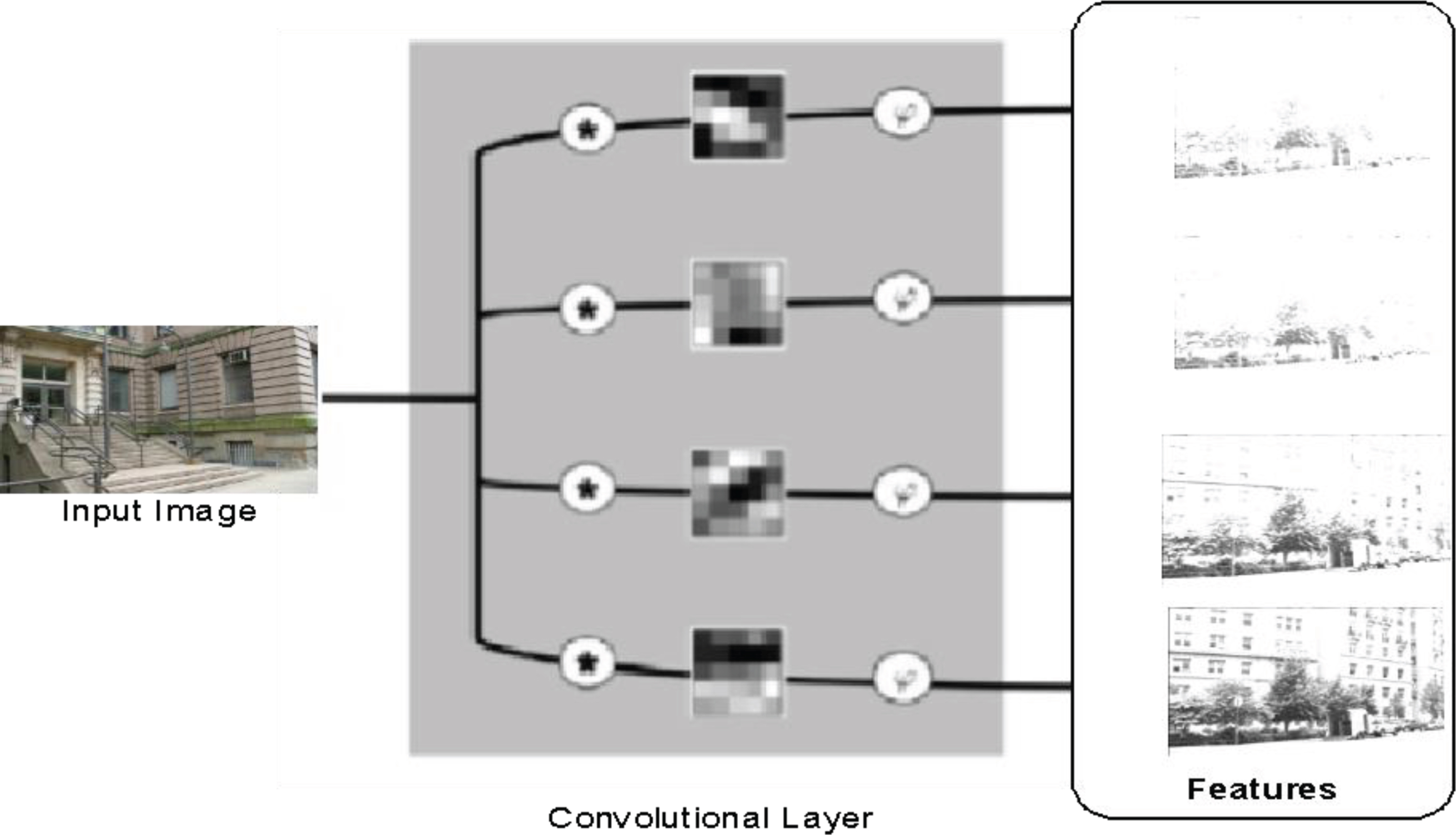
This paper presents a robust strategy is adopted for CMFD depends on deep learning. This strategy looking forward to build a new algorithm that achieve high performance, low testing time, and achieve low computational cost. Deep learning is one kinds of machine learning for supervised learning that the model understands and automatically do classification steps immediately to images. There are several advantages here in deep learning technique because of reduced contrast to forged images and the capability about more than one filters joined to the training step for discovering distinctive features. During training stage, all of filters will be pre-defined also their coefficients will be calculated. Essentially, during the training step, all weights from all layers arranged depending on the back-propagation technique with gradient descent algorithm [37]. Features will be trained automatically using the CNN in the training stage and presented to a classifier in the testing stage. CNN depends on multiple consecutive couples from convolutional (CNV) layer and pooling layer for producing discriminatory feature maps then followed by Fully Connected (FC) layers then classification layer [36]. Figure 2 illustrates the structure of CNN.

Fig.2

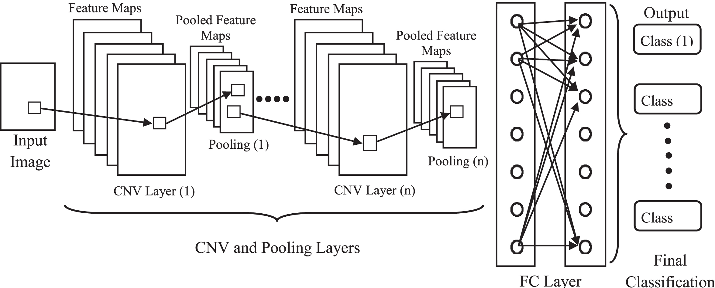
The structure of CNN.

3.1 Features Extractor Network

The proposed approach is based on a hybrid deep learning modality of ConvLSTM and CNN. The proposed model consists of three stages as shown in Fig. 3. The first stage is the pre-processing. This process is being carried out for two tasks. The first task is unifying the size of the input images to the same size, while the second task is converting the images to tensors. The second stage is the feature extraction stage. This stage is acquired to extract the features from the input images. The proposed model for feature extraction consists of one ConvLSTM layer, sequenced by three CNV layers and each one is followed by a pooling layer. This sequence of layers includes a ConvLSTM layer with 16 filters. Then, a combination of a CNV layer with a number of filters of 32 is followed by a max pooling layer. Furthermore, a combination of a CNV layer with number of filters of 64 and max pooling layer is carried out in addition to the final combination of 128 filter CNV layer with last max pooling layer. This sequence generates a feature map that represents the input image. This feature map is the input of the classification network. The classification network consists of two layers. The first layer is hybrid of GAP layer and FC layer. This layer handles the feature map generated by the sequence of ConvLSTM, CNV and pooling layers and converts it into a feature vector to be entered into the classification layer which is acquired to differentiate this feature vector into a predicted class.

Fig.3

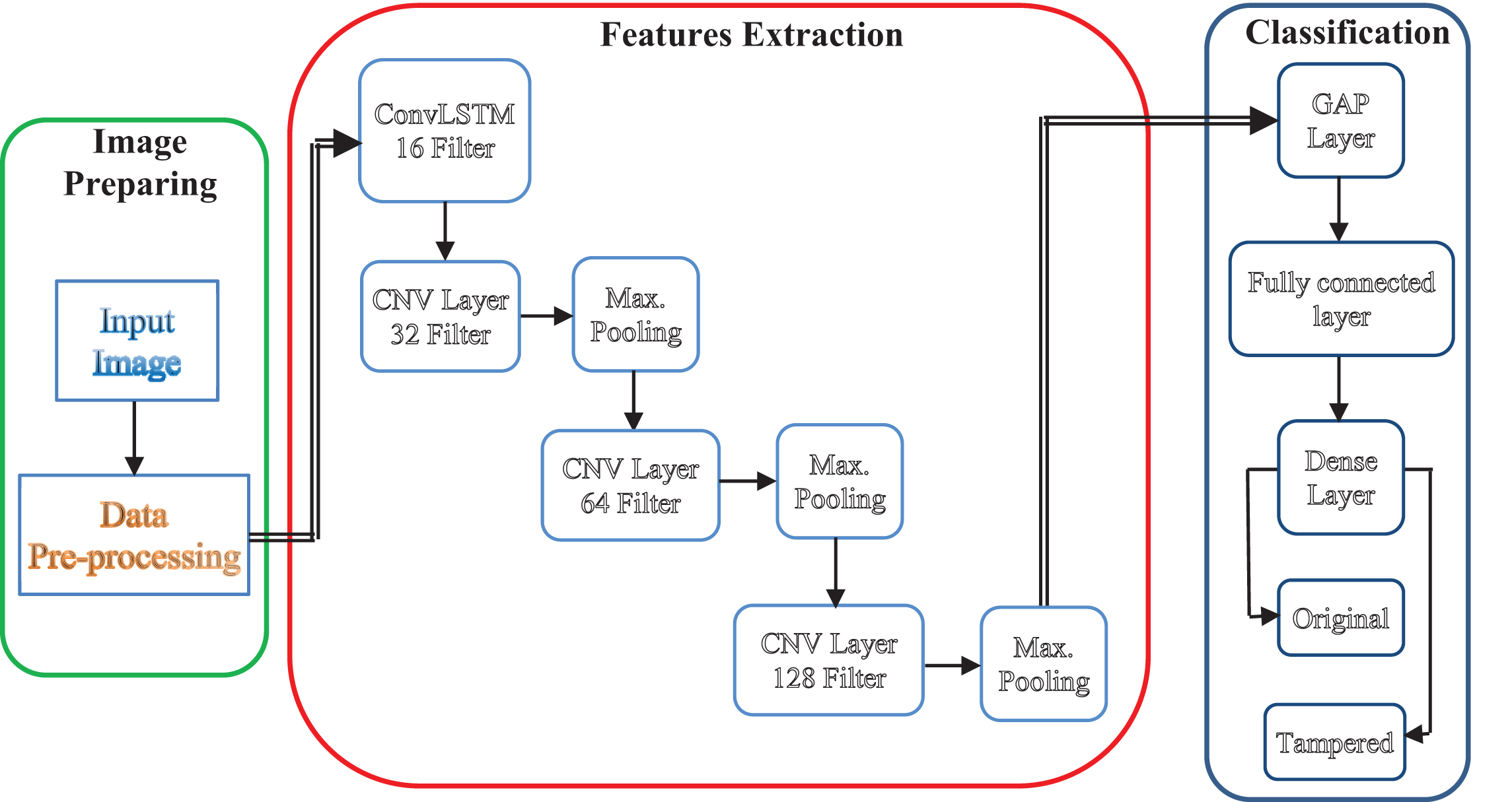
Layers of the proposed deep learning model.

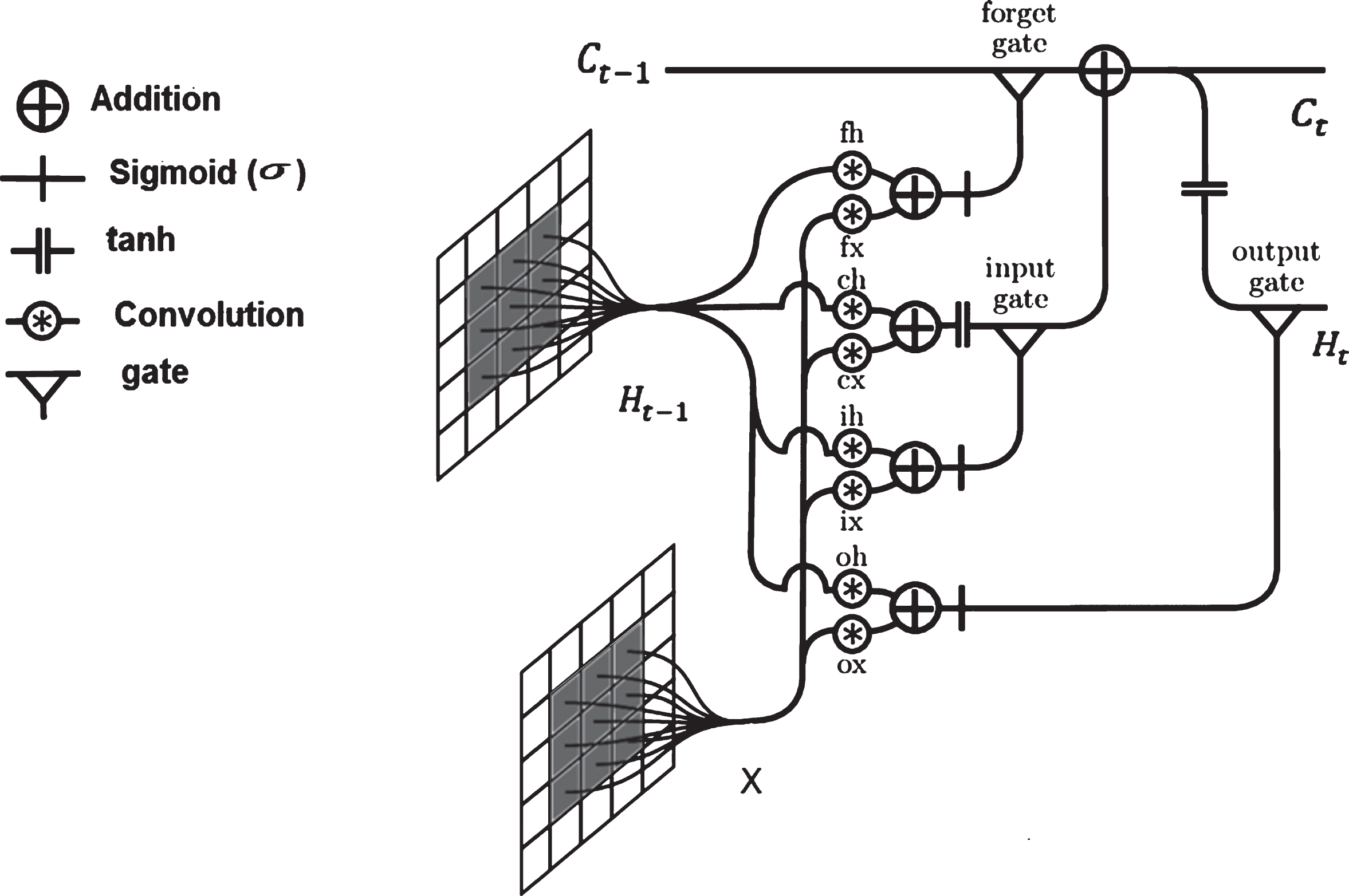
A) Convolutional Long Short-Term Memory (ConvLSTM)

There are three problems faces CNN using represents in can inability to handle sequence data, inability to memorize the previous output, and considers only the current input. LSTM is a special structure of Recurrent Neural Networks (RNN). As an RNN structure, it is proven that LSTM is stable and reliable for long-range dependencies in various research studies. But the basic disadvantage of this structure is the existence of several spatial data. To overcome these problems ConvLSTM is used. ConvLSTM replaces the FC layers in LSTM by CNV layers. If states are seen as the hidden representations of moving objects, larger transitional kernel of ConvLSTM should be capable of capturing faster motions, as shown in Fig. 4. To guarantee that the states with identical dimensions as inputs, padding is required prior using the convolution operation. All states are initialized to be zero prior the initial input which corresponds to “total ignorance” of the future [38 –40]. ConvLSTM has the capability of encoding the spatio-temporal information in its memory cell.

Fig.4

Architecture of ConvLSTM.

Where, i_t is the gate, C_t-1 is the status at the previous cell and it is hidden, f_t is the forget gate, H_t is the final state of the latest C_t, W is the weight of each connections, and o_t is the output gate. The values of the previous parameters are computed by the following equations: $i_{t} = σ (W_{xi} * X_{t} + W_{hi} H_{t - 1} + W_{ci} C_{t - 1} + b_{i})$ (1) $f_{t} = σ (W_{xf} * X_{t} + W_{hf} H_{t - 1} + W_{cf} C_{t - 1} + b_{f})$ (2) $C_{t} = f_{t} C_{t - 1} + i_{t} tanh (W_{xc} * X_{t} + W_{hc} H_{t - 1} + b_{c})$ (3) $o_{t} = σ (W_{xo} * X_{t} + W_{ho} H_{t - 1} + W_{co} C_{t} + b_{o})$ (4) $H_{t} = o_{t} tanh (C_{t})$ (5)

If states are seen as the hidden representations of moving objects, larger transitional kernel of ConvLSTM should be capable of capturing faster motions. To guarantee that the states with identical dimensions as inputs, padding is required prior using the convolution operation. All states are initialized to be zero prior the initial input which corresponds to “total ignorance” of the future.

B) The CNV Layer

CNV layer is a feature extraction layer which consists of a set of 2D digital filters. The values of these filters is initialized with low random weights. Then, the values of these weights are updated during the training process. The performed filters are expected to extract the features from the input images. This process generates a feature map with a depth of the filtered copies of the input image. Figure 5 shows an example of the convolutional process.

Fig.5

The convolution layer process.

The new value of a certain pixel (p_new) is the summation of the old surrounding pixels (p) multiplied by the applied filter elements (w). It can be calculated as follows: $p_{new} = \sum_{i \in s} p_{i} . w_{i}$ (6)

C) Activation Function

In order to evaluate the output of a certain layer, an activation function is carried out on the feature map generated from this layer. The result of the ReLU layers will use a linear activation function to the neuron output as illustrated in equation 7 where x is the input data. $f (x) = max (0, x)$ (7)

D) Pooling Layer

The pooling layer is a type of feature reduction methods which is used to reduce the dimensions of the feature map generated from the CNV layer. It is categorized into max pooling and mean pooling. The input feature map is segmented into windows. The max pooling splits each window into the maximum value among the included values in the window. On the other hand the mean pooling splits the window into the mean value of the included values in the window. Figure 6 shows an example for each pooling category.

Fig.6

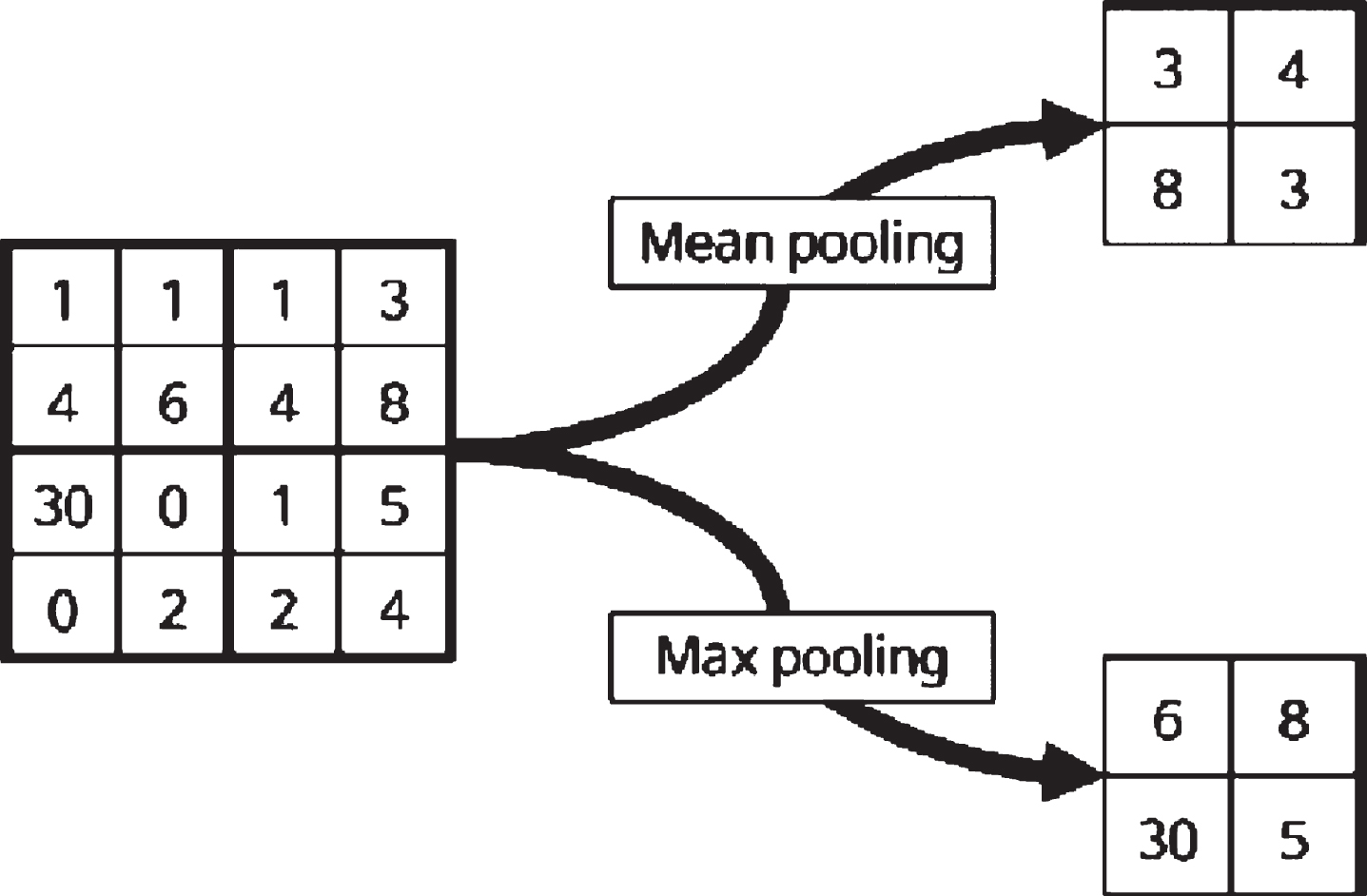
Pooling process using two different methods.

The max pooling layers have been performed in the proposed algorithm.

3.2 Classification network

The classification network consists of two layers. The first layer is a combination of the GAP layer and the FC layer. GAP layer handles the feature map generated by the sequence of ConvLSTM, CNV and pooling layers then converts it into a feature vector to be entered to the classification layer which is acquired to discriminate this feature vector to a predicted class. The FC layer is used to decease the feature vector size from 128 bytes to 64 bytes. This feature reduction acts as a protection stage against overfitting problem. Also, adding a second FC layer in this stage may cause features selection flounder. The discrimination process is carried out using an activation function. The activation function typically, soft-max sort of techniques had been used in this layer to obtain the classification result as illustrated in equation 8. On the other hand, the dense layer acts as organized output category. The dense layer evaluates the output to be either in the original class or in the forged class. $P (y = j | x) = \frac{e^{x^{T} w_{j}}}{\sum_{k = 1}^{K} e^{x^{T} w_{k}}}$ (8)

3.3 Back propagation

During the training process, it is required to update the weights of the proposed deep learning model. This update is evaluated by an optimization process. This paper performs Adam optimizer for this purpose [41]. In addition, the optimization process is carried out on a loss function. This function measures the error between the real and the predicted classes. This paper uses the cross entropy activation function. Using the other label convention t = (1 + y)/2, so that t∈ { 0, 1 }, the cross-entropy loss is defined as: $V (f (x), t) = - tln (f (x)) - (1 - t) \ln (1 - f (x))$ (9)

4 Results

In results section the valuation of the proposed algorithm outcomes had been presented. After results listing and discussing a comparison study with previous algorithms dealing with CMFD had been performed. To implement the proposed algorithm, a personal computer with Intel processor of core i7 8^th edition CPU, 4 GB GPU driver providing CUDA, 64 bits processor; RAM size of 8 GB, with an operating system of Windows 10 had been used. The proposed model had been performed by python 3.5 software tool in addition to Keras with TensorFlow software tools as backend toolkits. The summary of the proposed deep learning algorithm layers processing is shown in Table 1.

Table 1
Summery of proposed deep learning model

Layer Type Output Shape

Batch Normalization (Number of patterns, 224, 224, 3)

Reshape to ConvLSTM (Number of patterns, 224, 224, 3)

ConvLSTM (Number of patterns, 224, 224, 16)

Reshape to Conv. (Number of patterns, 224, 224, 16)

Conv. (Number of patterns, 222, 222, 32)

The process of Pooling (Number of patterns, 111, 111, 32)

Conv. (Number of patterns, 109, 109, 64)

The process of Pooling (Number of patterns, 54, 54, 64)

Conv. (Number of patterns, 52, 52, 128)

The process of Pooling (Number of patterns, 26, 26, 128)

The Global Average Layer (Number of patterns, 128)

The Dense process (Number of patterns, 2)

Layer Type	Output Shape
Batch Normalization	(Number of patterns, 224, 224, 3)
Reshape to ConvLSTM	(Number of patterns, 224, 224, 3)
ConvLSTM	(Number of patterns, 224, 224, 16)
Reshape to Conv.	(Number of patterns, 224, 224, 16)
Conv.	(Number of patterns, 222, 222, 32)
The process of Pooling	(Number of patterns, 111, 111, 32)
Conv.	(Number of patterns, 109, 109, 64)
The process of Pooling	(Number of patterns, 54, 54, 64)
Conv.	(Number of patterns, 52, 52, 128)
The process of Pooling	(Number of patterns, 26, 26, 128)
The Global Average Layer	(Number of patterns, 128)
The Dense process	(Number of patterns, 2)

4.1 Datasets description

The extreme challenged or famous databases in CMFD algorithms valuation are MICC-F220 [29], MICC-F2000 [29], MICC-F600 [42], and newly SATs-130 [43]. The details descriptions of these evaluation databases are illustrated in Table 2.

Table 2
The specifications of datasets MICC-F220, MICC-F2000, MICC-F600, and SATs-130

Dataset Composition Size of Images Size of Tampered Region

MICC-F220 220 images divided into 110 forged images and 110 original images. Varied from 722×480 to 800×600 pixels The forged region is 1.2% of the whole image.

MICC-F2000 2000 images divided into 700 forged images and 1300 original images. 2048×1536 pixels The forged region is 1.12% of the whole image.

MICC-F600 600 images divided into 152 forged images and 448 original images. Varied from 800×532 to 3888×2592 pixels The forged region size varies from one image to another.

SATs-130 96 images divided into 48 forged images and 48 original images. Varied from 1024×683 to 3264×2448 pixels The forged region size varies from one image to another.

Combined dataset 2916 images divided into 1010 forged images and 1906 original images. Varied from 722×480 to 3888×2592 pixels The forged region size varies from one image to another.

Dataset	Composition	Size of Images	Size of Tampered Region
MICC-F220	220 images divided into 110 forged images and 110 original images.	Varied from 722×480 to 800×600 pixels	The forged region is 1.2% of the whole image.
MICC-F2000	2000 images divided into 700 forged images and 1300 original images.	2048×1536 pixels	The forged region is 1.12% of the whole image.
MICC-F600	600 images divided into 152 forged images and 448 original images.	Varied from 800×532 to 3888×2592 pixels	The forged region size varies from one image to another.
SATs-130	96 images divided into 48 forged images and 48 original images.	Varied from 1024×683 to 3264×2448 pixels	The forged region size varies from one image to another.
Combined dataset	2916 images divided into 1010 forged images and 1906 original images.	Varied from 722×480 to 3888×2592 pixels	The forged region size varies from one image to another.

The challenged attacks in MICC-F600 dataset are divided into four levels with different forgery attacks [42]. The proposed algorithm had been tested directly with datasets MICC-F600, MICC-F2000 and MICC-F220. While dataset SATs-130 is composed of minimal number of images (96 images) which collide with the nature of deep learning algorithms. Training step in deep learning algorithms needs large datasets to be able to correctly extract features maps and build system behavior. Using small datasets may cause overfitting problem. Also, overfitting problem happened if the training periods are expanded to the scale which the deep learning algorithm mayn’t accurately produce the feature plans. For solving this problem, MICC-F220, MICC-F2000, MICC-F600, and SATs-130 datasets have been merged to build a comprehensive combinational database. Datasets combination simply allow the algorithm to test SATs-130 dataset and growing the database dimensionality to popularize the assessment operation. The new dataset composed of 2916 images splitted into 1010 forged and 1906 authentic and changed between (722×480) and (3888×2592) with changing dimensionalities of forged parts as illustrated in Table 2. Figure 7 shows several examples of original and forged images used in different datasets.

Fig.7

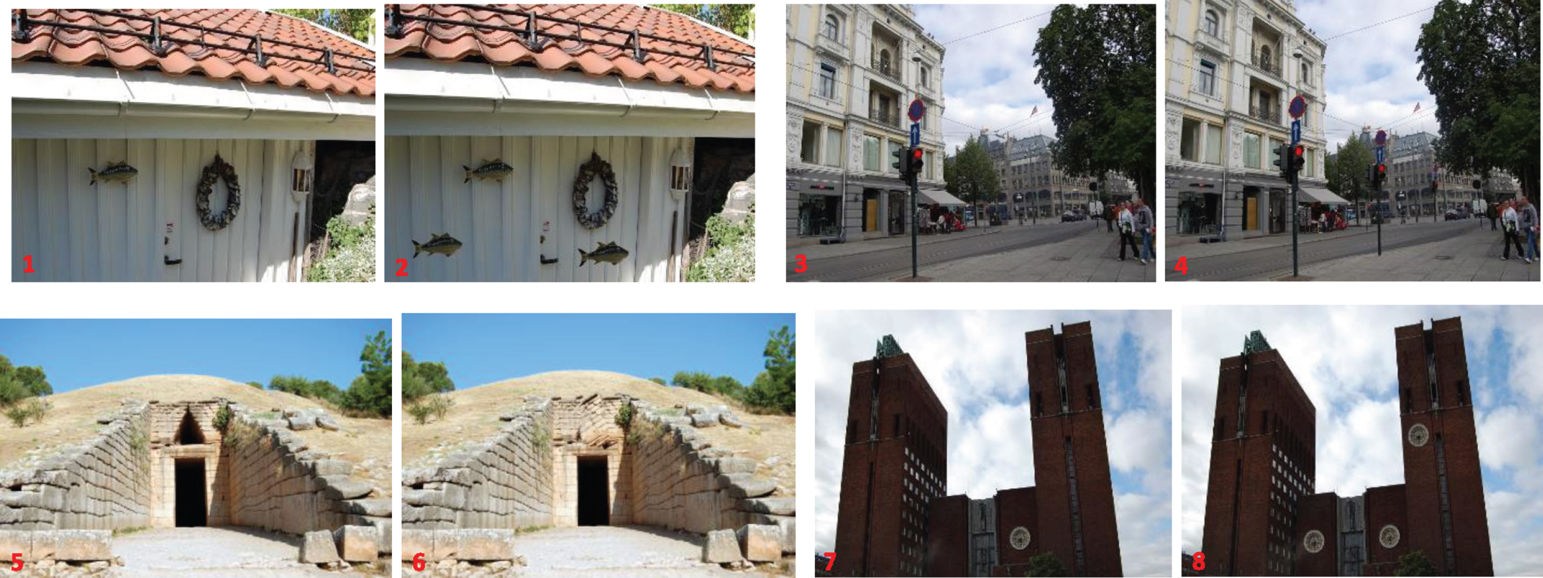
Examples of images used in different datasets: image 1, 3, 5, and 7 are original image but images 2, 4, 6, and 8 are their forged images.

4.2 Evaluation metrics

Estimating the strength of the deep Learning ConvLSTM algorithm is performed by using accuracy, True Positive Rate (TPR), False Positive Rate (FPR), False Negative Rate (FNR) and True Negative Rate (TNR). The equations of these performance metric parameters are presented in Equations 10, 11, 12, 13, and 14:

$\begin{matrix} Accuracy = \frac{No . of correctly detected images}{Total No . of images} \\ \times 100 = \frac{(T_{N} + T_{P})}{(T_{P} + F_{P} + T_{N} + F_{N})} \times 100 \end{matrix}$ (10) $TPR = T_{P} / (T_{P} + F_{N}) = (1 - FNR)$ (11) $FPR = F_{P} / (F_{P} + T_{N}) = (1 - TNR)$ (12) $FNR = F_{N} / (F_{N} + T_{P})$ (13) $TNR = T_{N} / (T_{N} + F_{P})$ (14)

Where

False Negative (F_N) represents the quantity of tampered images which had been wrong discovered as authentic images.

True Positive (T_P) represents the quantity of tampered images which had been correctly discovered as tampered images.

True Negative (T_N) represents the quantity of authentic images which had been correctly discovered as authentic images.

False Positive (F_P) represents the quantity of authentic images which had been wrong discovered as tampered images.

The Logarithmic loss (Log Loss) parameter denotes the false classifications and used with multiple class classification. For N patterns related to M categorizes, the Log Loss is presented in the following equation: $LogLoss = \frac{- 1}{N} \sum_{a = 1}^{N} \sum_{b = 1}^{M} Z_{ab} . log (p_{ab})$ (15) where Z_ab references if pattern (a) relate to class (b) or not and p_ab references the prospect of that pattern (a) related to quantity (b). When Log Loss is near to zero, which means a higher values of accuracy.

In addition, Testing Time (TT) is also used to evaluate the deep learning ConvLSTM model and to examine it with different models. The TT is the average time needed to test the images for the number of rounds equal (k) during the testing process. Also, Learning Time is not counted because this step is only performed offline for one time.

4.3 The results

The paper proposed new strategy of deep learning modality for image forgery detection process. The proposed model consists of a hybrid architecture of ConvLSTM and CNN layers. The proposed deep learning model is carried out on several datasets including MICC-F220, MICC-F600 and MICC-F2000 as well as a combination between them with adding of SATs-130 dataset. The motivation of the simulation experiments is to achieve an optimum model regarding the complicity and the testing time. Furthermore, k-fold cross-validation technique had been performed to evaluate the proposed algorithm.

This model based first on learning step which will be iterated (k) to obtain the variety among the examined images and achieve powerful estimation by totally examining the databases. This model continues by splitting the database in a random way into (k) categories (folds) with nearly same dimensionality. The proposed model used (k-1) classes for training, and the residual classes used for testing. There are (k) iterations that used for training and testing. The proposed algorithm used a 5-fold cross-validation mechanism. So, about 80% of the images in the database had been selected in a random way for training but the residual 20% had been used for testing, for all five iterations. In every iteration, other 20% of the images will be used for testing than the old 20% of images.

The experiments consist of five trails at 15, 25, 50, 75 and 100 training epochs and recording of the TPR, FPR, TNR, FNR and accuracy at each epoch. In addition, a record of the testing time is considered in the simulation experiments. Tables 3 to 7 summarizes the simulation results at each epoch for all datasets. It can be observed that the increment of the quantity of epochs leads to growing in the execution of the proposed model. In addition, the execution of the proposed approach differs from such a dataset to another. So, there are two restrictions effect on the execution of the proposed model. The first is the quantity of the training epochs, while the second restriction is the construction nature of the dataset on which the proposed model is carried out.

Table 3
The results of performing the proposed model for different datasets at 15 epochs

Datasets\Metric TPR% FPR% FNR% TNR% Accuracy% LogLoss% TT (Sec)

MICC-F220 100 10.9 zero 89.1 93.9 6.1 1.322

MICC-F600 55 9.7 45 90.3 76.5 23.5 1.3131

MMIC-2000 99.4 11.9 0.6 88.1 95 5 4.1680

Combined Dataset 79.1 9.5 20.9 88.5 81.5 18.5 7.0133

Datasets\Metric	TPR%	FPR%	FNR%	TNR%	Accuracy%	LogLoss%	TT (Sec)
MICC-F220	100	10.9	zero	89.1	93.9	6.1	1.322
MICC-F600	55	9.7	45	90.3	76.5	23.5	1.3131
MMIC-2000	99.4	11.9	0.6	88.1	95	5	4.1680
Combined Dataset	79.1	9.5	20.9	88.5	81.5	18.5	7.0133

Table 4

The results of performing the proposed model for different datasets at 25 epochs

Datasets\Metric	TPR%	FPR%	FNR%	TNR%	Accuracy%	LogLoss%	TT (Sec)
MICC-F220	100	10.9	zero	89.1	93.9	6.1	1.2959
MICC-F600	70.6	5.9	29.4	94.1	86.3	13.7	1.3207
MMIC-2000	98.2	6.3	1.8	93.7	96.6	3.4	4.2450
Combined Dataset	93.2	10.5	6.8	89.5	91.9	8.1	7.0912

Table 5

The results of performing the proposed model for different datasets at 50 epochs

Datasets\Metric	TPR%	FPR%	FNR%	TNR%	Accuracy%	LogLoss%	TT (Sec)
MICC-F220	100	4.5	zero	95.5	97.7	2.3	1.2963
MICC-F600	74.5	10.2	35.5	89.5	87.5	12.5	1.3256
MMIC-2000	98.2	5.7	1.8	94.3	96.8	3.2	4.1991
Combined Dataset	99.2	13.4	0.8	86.6	94.1	5.9	7.1257

Table 6

The results of performing the proposed model for different datasets at 75 epochs

Datasets\Metric	TPR%	FPR%	FNR%	TNR%	Accuracy%	LogLoss%	TT(Sec)
MICC-F220	100	3	zero	97	98.8	1.2	1.2993
MICC-F600	90.1	1.8	9.9	98.2	96.2	3.8	1.3714
MMIC-2000	100	5.5	zero	94.5	98	2	4.1555
Combined Dataset	94.4	6.6	5.6	93.4	94	6	7.1126

Table 7

The results of performing the proposed model on different datasets at 100 epochs

Datasets\Metric	TPR%	FPR%	FNR%	TNR%	Accuracy%	LogLoss%	TT (Sec)
MICC-F220	100	zero	zero	100	100	Zero	1.2939
MICC-F600	97.6	1.1	2.4	98.99	98.89	1.11	1.3841
MMIC-2000	100	1.9	zero	98.1	98.14	1.86	4.2631
Combined Dataset	100	2.95	zero	97.05	97.13	2.87	7.2993

The testing accuracy of MICC-F220 dataset achieved an accuracy of 93.9%, 93.9%, 97.7%, 98.8% and 100% for 15 epochs, 25 epochs, 50 epochs, 75 epochs and 100 epochs, respectively. In addition, MICC-F600 achieved an accuracy from 76.5 % at 15 epochs and increasing to 98.89% at 100 epochs. Furthermore, MICC-F2000 achieved an accuracy in the range of 95% to 98.14%. The combined dataset achieved an accuracy range from of 81.5% at 15 epochs and 97.13% at 100 epochs.

Tables 3, 4, 5, 6, and 7 present the results of the performance metric parameters for the different four datasets at epochs 15, 25, 50, 75, and 100 respectively. The results depicted from the tables present that the accuracy, TPR, and TNR raise nearly to 100% at number of epochs equal to 100. Opposite of that, FPR and FNR minimized nearly to zero at also when number of epochs equal to 100. Furthermore, the TT reduced to minimal with increasing the number of epochs.

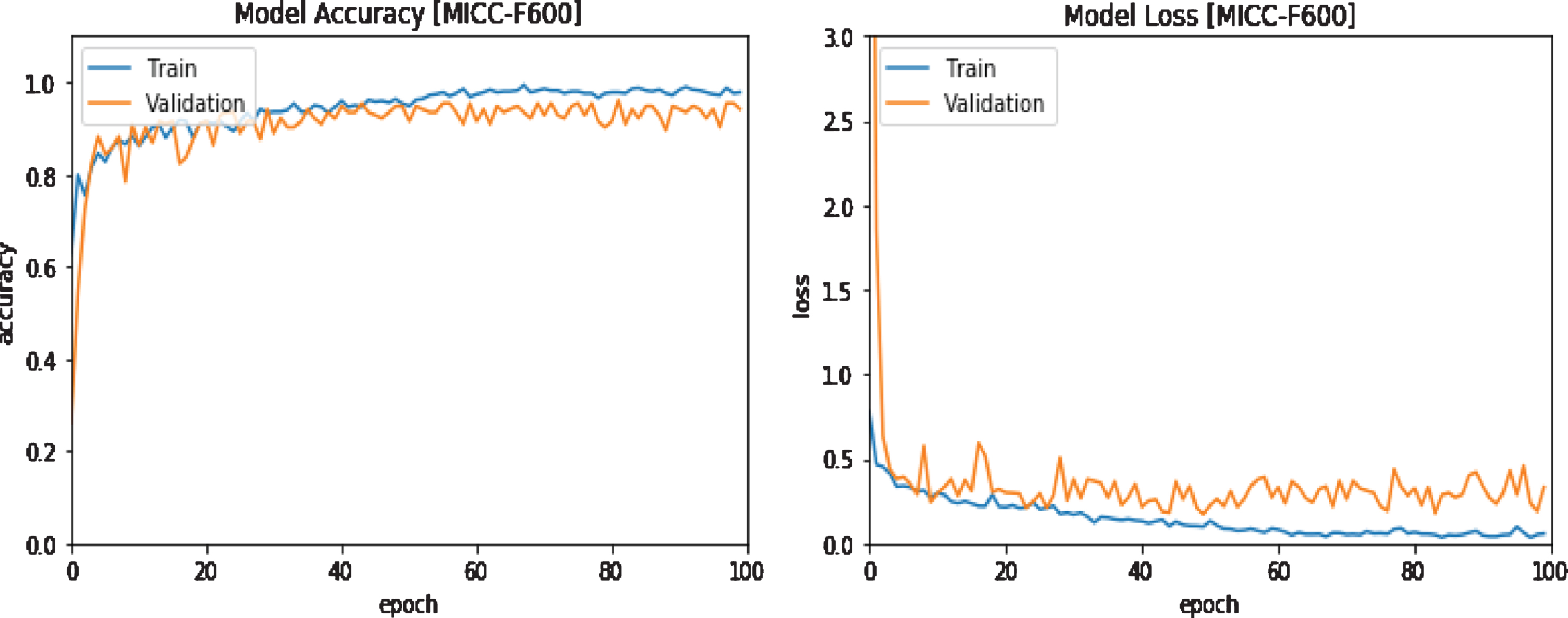
It can be noticed that the previous results presented the quantity of training parts reflects a high effect on the total model execution. Also, it is noticed that the best results appear at 100 epochs. Figures 8, 9, and 10 present the training and validation curves for the MICC-F220, MICC-F600 and MICC-F2000 databases. In addition, the combined database, presented in Fig. 11, expounds the training and validation curves. The output explains that the testing accuracy raised and set at 100%, 98.89%, 98.14%, and 97.13% for MICC-F220, MICC-F600 and MICC-F2000, and combined databases at 100 epochs. Whereas the testing loss decreased and set at zero, 1.11%, 1.86%, and 2.87% for MICC-F220, MICC-F600 and MICC-F2000, and combined databases at 100 epochs at 100 epochs.

Fig.8

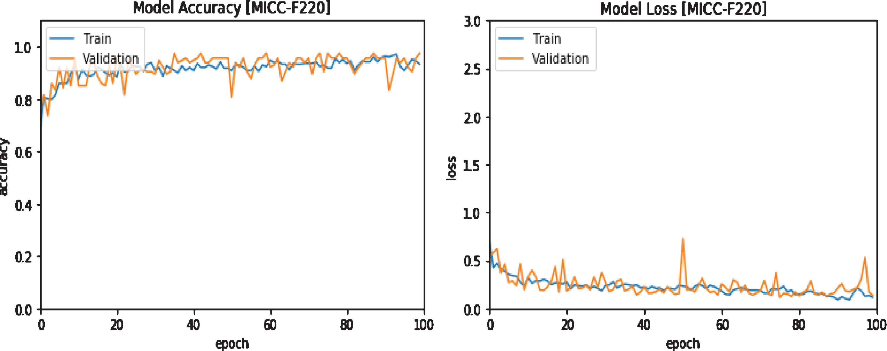
Accuracy and LogLoss of the proposed approach of MICC-F220 database at 100 epochs.

Fig.9

Accuracy and Log Loss of the proposed approach of MICC-F2000 database at 100 epochs.

Fig.10

Accuracy and Log Loss of the proposed approach of MICC-F600 database at 100 epochs.

Fig.11

Accuracy and Log Loss of the proposed approach of the combinational database at 100 epochs.

The proposed algorithm (ConvLSTM) had various identifiers which influence the output in either Accuracy or testing time. These identifiers are the quantity of the data used for the training (which related to the dimensionality of the used databases), the quantity of the data used as an input to the model, the quantity of hidden layers of the model, and the quantity of the epochs that will be selected. At making the identifiers of quantity of the data used for the training, the quantity of the data used as an input, and the quantity of hidden layers of the model are constant. So, the single remaining identifier which influences the time of testing is the quantity of the selected epochs.

It was found that there is a common influence between is the quantity of the selected epochs and the time needed by the algorithm to achieve the ideal map of feature. The needed time by the algorithm to achieve the ideal map of feature permits it to achieve the top performance. By selecting an exact quantity of epochs, the ideal map of feature will be extracted. In addition to the quantity of epochs, overfitting will be happened. Furthermore, reducing the quantity of epochs than the selected amount will make the model failed to extract the ideal map of features. Therefore, the quantity of selected epochs influences the TT if the rest of the identifiers are remained constant.

Figure 12 illustrates a comparison study among the accuracy of the proposed approach for each database at several epochs while Fig. 13 illustrates the optimal accuracy representation for each dataset. The simulation results reveal that the proposed algorithm may be considered as a reliable and applicable technique for CMFD. For example, at MICC-F220 dataset the proposed algorithm achieved an accuracy of 100% with a testing time of 1.2939 seconds for 44 images represents 20% of the overall dataset size tested in one k-fold round. This means that the single image takes 29.4 m second for testing process which represents a very low testing time with a reliable accuracy of detection. Figure 14 shows the average TT for each dataset at 100 epochs.

Fig.12

Accuracy comparisons of the proposed model for each dataset at different epochs.

Fig.13

Optimal accuracy of detection for different datasets.

Fig.14

The average of TT for different datasets at 100 epochs.

Furthermore, The Receiver Operating Characteristic (ROC) is utilized also as evaluation metric. Within a ROC curve, the TPR (sensitivity) is represented as a function of the FPR (specificity) at distinct cut-off points. Every point on the ROC curve illustrates a sensitivity/specificity pair congruent to a specific decision threshold. A test with good discrimination (no overlapping in the two distributions) implies that the ROC curve (blue curve) surpasses through the upper left corner (100% sensitivity, 100% specificity). So, on the ROC curve, the nearer to the upper left corner is the higher values of overall accuracy of the test. Figure 15 shows the ROC curves of the proposed algorithm for MICC-F220, MICC-F600 and MICC-F2000 as well as the combined dataset.

Fig.15

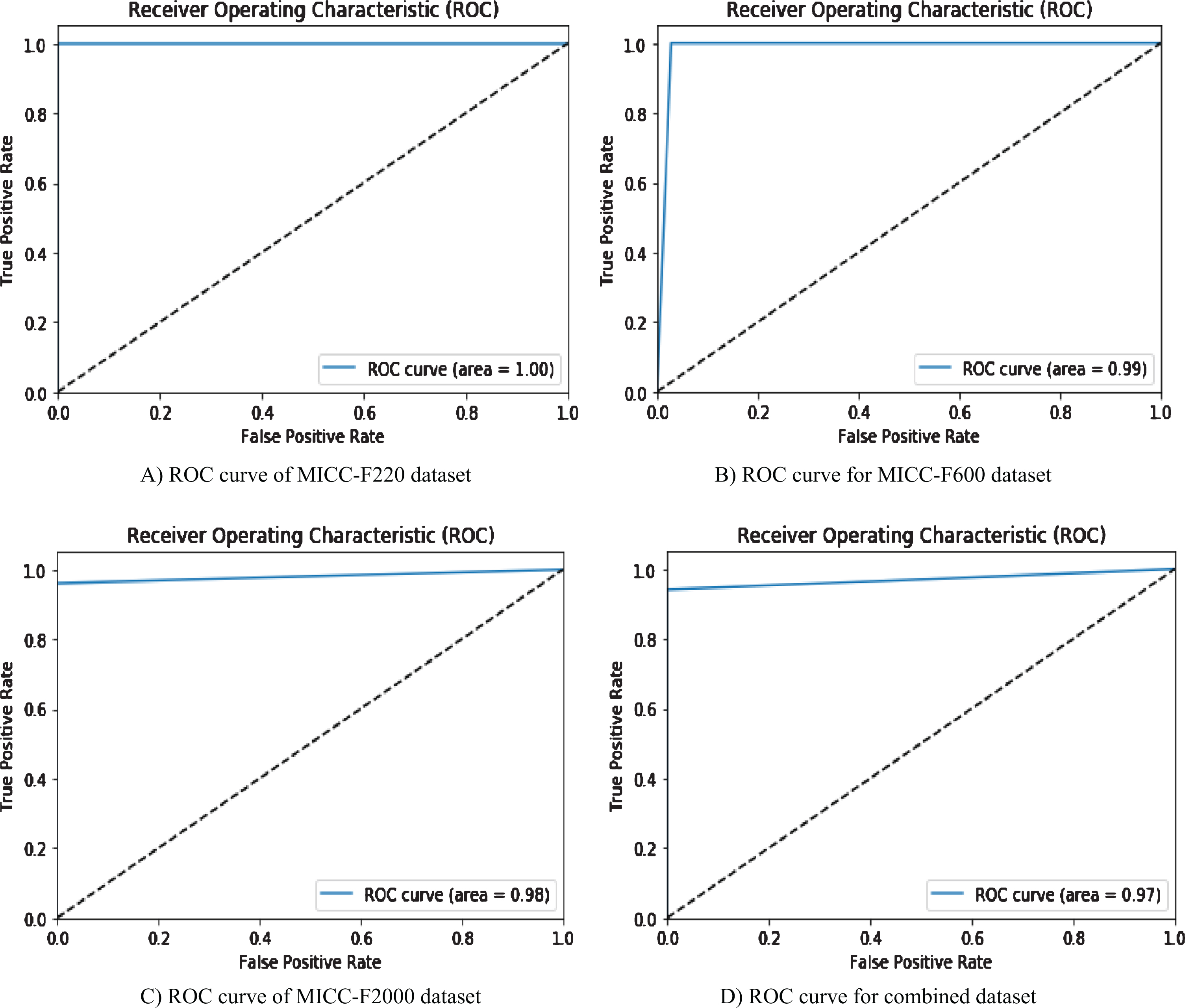
ROC curves of the proposed algorithm for different datasets.

A major question has been raised in the way of proving the proposed algorithm efficiency. Why using hybrid of ConvLSTM and CNN is more efficient than using CNN or ConvLSTM alone? The proposed algorithm uses the hybrid models, including ConvLSTM and CNN, instead of using CNN or ConvLSTM alone in order to achieve the advantages of each model. The CNN model produces features with low processing time, on the other hand, the ConvLSTM solves the problem of vanishing gradation which appears in CNN model in back propagation step. So, the proposed algorithm can achieve high performance with low processing time and stability progressing in both learning and testing process. Table 8 shows the performance results of the ConvLSTM model for different datasets at only 100 epochs. Table 8 shows that using ConvLSTM results isn’t efficient comparing with using hybrid of ConvLSTM and CNN. In this experiment, 100 epochs have been performed comparing to the best results obtained from the proposed algorithm also at 100 epochs.

Table 8

The results of performing the ConvLSTM model for different datasets at 100 epochs

Datasets\Metric	TPR%	FPR%	FNR%	TNR%	Accuracy%	LogLoss%	TT(Sec)
MICC-F220	78.95	19.05	21.05	80.95	84.21	15.79	3.3822
MICC-F600	64.29	12.61	35.71	87.39	85.62	14.38	4.3516
MMIC-2000	92.42	14.12	7.58	85.88	91.21	8.79	11.5654
Combined Dataset	87.50	20.79	12.50	79.21	85.01	14.99	33.8415

The results of the accuracy ranged from about 84.21% and 91.21% for different datasets compared with the hybrid model that ranged from 97.13% to 100%. Also, from Table 8, the TPR ranged from 64.29% to 92.42% compared to variation from 97.6% to 100% for different datasets in the proposed algorithm. In addition, the TNR resulted from using ConvLSTM only is varied from 79.21% to 87.39% compared to the TNR variation of 97.05% to 100% resulting from using the hybrid model in the proposed algorithm. Figures 16, 17, 18, and 19 present the training and validation curves for the MICC-F220, MICC-F600, MICC-F2000 and the combined database. These curves represent the training and validation curves resulting from using the ConvLSTM model only. Another major notice appears in TT, where the TT is about quadruple more than its values when performing the hybrid solution when performing ConvLSTM model. The TT ranges from 3.3822 seconds to 33.8415 seconds when using the ConvLSTM only compared to the variation from 1.2939 seconds to 7.2993 seconds in the proposed algorithm.

Fig.16

Accuracy and LogLoss of the ConvLSTM model only on MICC-F220 database at 100 epochs.

Fig.17

Accuracy and LogLoss of the ConvLSTM model only on MICC-F600 database at 100 epochs.

Fig.18

Accuracy and LogLoss of the ConvLSTM model only on MICC-F2000 database at 100 epochs.

Fig.19

Accuracy and LogLoss of the ConvLSTM model only on combinational database at 100 epochs.

Figures 16, 17, 18, and 19 show that the ConvLSTM model has the advantage of maximizing the vanishing degradation. It is appeared from figures that there is no degradation in the progressing curve but, on the other hand, it takes more processing time and doesn’t achieve high performance as shows in Table 8. The CNN model has these missing advantages, so hybrid ConvLSTM and CNN have been performed. The proposed algorithm can achieve high performance with low processing time and stability (without degradation) in both learning and testing process progressing.

4.4 Comparison study with previous algorithms

A comparison study among previous strong models with the proposed model that use different detection techniques will be represented. The algorithms used in this comparison are listed as Amerini et al. [29], Amerini et al. [42], Mishra et al. [44], Kaur et al. [45], Elaskily et al. [36], Elaskily et al. [46], and Wankhade et al. [47]. The algorithms in [29], [42], [36], and [46] had been executed on the PC itself which had been utilized for experimenting the proposed model. Nevertheless, the model in [44] had been simulated other PC with specifications of Intel core i5 micro-processor with 64-bits and the used operating system was Windows 8.1 and setting up the MATLAB version R2013a software. The other models, Kaur et al. [45] and Wankhade et al. [47] didn’t specify the utilized software and hardware.

For deep learning algorithms, it is familiar that the training stage is performed only one time to build the classification scheme behavior. The moment that the scheme had been done, it will be served to do the classification step with higher speed. So, the TT, which calculated in the testing stage, is compared with the execution time of the other traditional algorithms and with TT of other deep learning algorithms.

Tables 8, 9, and 10 give a brief about the results of the comparison study. The tables illustrate that the proposed model (ConvLSTM) based on deep learning gives high execution results compared to all other traditional algorithms in both detection accuracy and TT. Comparing with the deep learning algorithm in Elaskily et al. [36], the proposed deep learning ConvLSTM based algorithm accuracy can reach approximately to the same accuracy. For example, the accuracy is 100%, 98.89%, 98.14%, 97.13% for datasets MICC-F220, MICC-F600, MICC-F2000, and combined databases consequently for the proposed algorithm comparing with 100% for all datasets for Elaskily et al. [36] algorithm. The major weight for out proposed model is the TT, where it is reach to a very minimum values comparing with other traditional algorithms or other deep learning algorithm. The TT effects on the computational efficiency, speed, and computing resources which it is in the best interest of the proposed algorithm. From Table 8 it is clear that TT decreased from 14 seconds in its minimum value in Elaskily et al. [36] to 1.29 seconds for the proposed algorithm for dataset MICC-F220. Also, TT decreased from one minute and 19 seconds in its minimum value in Elaskily et al. [36] to 4.26 seconds for the proposed algorithm for dataset MICC-F2000 as shown in Table 9. In addition, TT decreased from 24 seconds in its minimum value in Elaskily et al. [36] to 1.38 seconds for the proposed algorithm for dataset MICC-F600 as shown in Table 10.

Table 9
Comparison among the proposed approach and other published models for MICC-F220 database

Metric\Algorithm The Proposed Elaskily Amerini Amerini Mishra Kaur Elaskily Wankhae

Approach et al. [36] et al. [29] et al. [42] et al. [44] et al. [45] et al. [46] et al. [47]

TPR % 100 100 100 100 73.64 97.27 100 100

FPR % Zero Zero 8 6 3.64 7.27 1.80 3.63

FNR % Zero Zero Zero Zero 26.36 2.73 Zero Zero

TNR % 100 100 92 94 96.36 92.73 98.20 96.37

TT (mm:ss) 0 : 1.29 0 : 14 24 : 13 17 : 05 0 : 2.85 N/A 2 : 48 N/A

Metric\Algorithm	The Proposed	Elaskily	Amerini	Amerini	Mishra	Kaur	Elaskily	Wankhae
TPR %	100	100	100	100	73.64	97.27	100	100
FPR %	Zero	Zero	8	6	3.64	7.27	1.80	3.63
FNR %	Zero	Zero	Zero	Zero	26.36	2.73	Zero	Zero
TNR %	100	100	92	94	96.36	92.73	98.20	96.37
TT (mm:ss)	0 : 1.29	0 : 14	24 : 13	17 : 05	0 : 2.85	N/A	2 : 48	N/A

Table 10

Comparison among the proposed approach and other published models for MICC-F2000 database

Metric\Algorithm	The Proposed	Elaskily	Amerini	Amerini	Elaskily
Approach	et al. [36]	et al. [31]	et al. [47]	et al. [46]
TPR %	100	100	93.42	94.86	98.40
FPR %	1.9	Zero	11.61	9.15	6.35
FNR %	Zero	Zero	6.58	5.14	1.60
TNR %	98.1	100	88.39	90.85	93.65
TT (mm:ss)	0 : 4.26	01 : 19	312 : 18	180 : 15	46 : 58

5 Result discussion

There are different identifiers which influence the output in both of Accuracy and testing time in the proposed approach such as the amount of training data, the quantity of the data used as an input to the model, the quantity of hidden layers of the model, and the quantity of the epochs that will be selected. At making the identifiers of quantity of the data used for the training, the quantity of the data used as an input, and the quantity of hidden layers of the model are constant. So, the single remaining identifier which influences the time of testing is the quantity of the selected epochs.

From the previous results, where the accuracy had been measured at different number of epochs, it had been observed that the output which the a mounts of the accuracy, TPR, and TNR of the proposed algorithm increased to reach near to 100% when using number of epochs equal 100. At the same time, FPR and FNR reduced near to zero also at number of epochs equal 100 and the TT time reduced as the quantity of epoch’s increase. Also, the accuracy of the training and validation curves changed from 97% to 100% for the four datasets at number of epochs equal 100 and the test loss differ from zero to nearly 3% for the four datasets at number of epochs equal 100.So, the best results appear at 100 epochs.

A comparison study among the proposed algorithm and several other previous algorithms. The proposed algorithm gives high accuracy reached to 100% for some datasets with lowest TT time nearly 1 second for some datasets when compared to the other previous algorithms as illustrated in Tables 9, 10, and 11.

Table 11
Comparison among the proposed approach and other published models for MICC-F600 database

Metric\Algorithm The Proposed Elaskily Amerini Amerini Elaskily

Approach et al. [39] et al. [34] et al. [50] et al. [46]

TPR % 97.6 100 69.20 81.60 94.50

FPR % 1.1 Zero 12.50 7.27 11.35

FNR % 2.4 Zero 30.80 18.40 5.5

TNR % 98.99 100 87.50 92.73 88.65

TT (mm:ss) 0 : 1.38 0 : 24 115 : 00 76 : 21 17 : 37

Metric\Algorithm	The Proposed	Elaskily	Amerini	Amerini	Elaskily
TPR %	97.6	100	69.20	81.60	94.50
FPR %	1.1	Zero	12.50	7.27	11.35
FNR %	2.4	Zero	30.80	18.40	5.5
TNR %	98.99	100	87.50	92.73	88.65
TT (mm:ss)	0 : 1.38	0 : 24	115 : 00	76 : 21	17 : 37

6 Conclusions and future work

A deep learning algorithm based on hybrid ConvLSTM and CNN for CMFD was presented in this paper. The basic objective of this paper is to build and improve the deep learning classification model for classifying suspected digital image forgery into original class and forged class. The proposed algorithm is looking forward to building a new model that will deliver increased performance, minimal testing time, and achieve low computational cost. The development of the suggested forgery detection system is discussed in three layers; the pre-processing layer, the feature extraction layer, and the classification layer. In the feature extraction layer, the proposed approach is based on a new development by constructing a serial sequence of CovLSTM, CNV layer, and pooling layer that accelerates the classification process. In the evaluation process, various challenged datasets have been used such as MICC-F220, MICC-F2000, MICC-F600, and SATs-130 databases. For more generalization and different testing performing issues such as overfitting problem, a combined dataset is collected and used for the proposed algorithm testing. The testing results showed that the highest accuracy had been obtained with 100 training epochs. The Accuracy reaches 100%, 98.89%, 98.14%, and 97.13% for databases MICC-F220, MICC-F2000, MICC-F600, and combined databases. While the system loss represented in LogLoss parameter minimized to zero, 1.11%, 1.86%, and 2.87% for databases MICC-F220, MICC-F2000, MICC-F600, and combined database. In addition, the results presented that the TT of the proposed model had been minimized to a very low level. The average TT reaches 1.29, 1.38. 4.26, and 7.29 seconds for datasets MICC-F220, MICC-F2000, MICC-F600, and combined database which means that the proposed approach is characterized by its speed in addition to accuracy.

In the future work, the proposed algorithm will be applied to other challenged datasets such as CASIA, COVERAGE, and CoMoFoD. Additionally, a CMFD system will be applied on cloud-based deep learning.

Footnotes

Acknowledgments

This work was funded by the University of Jeddah, Saudi Arabia, under grant No. (UJ-04-18-ICP). The authors, therefore, acknowledge with thanks the University technical and financial supports.

References

Guojuan

, Dianji

, An Overview of Digital Watermarking in Image Forensics, Fourth International Joint Conference on Computational Sciences and Optimization, 10.1109/cso.2011.85, 2011.

David

, Divya

, Image Authentication Techniques and Advances Survey, COMPUSOFT, An international journal of advanced computer technology IV(IV) (2015).

Elaskily

M.A.

, Aslan

H.K.

, Abd El-Samie

F.E.

, Elshakankiry

O.A.

, Faragallah

O.S.

and Dessouky

M.D.

, Comparative study of copy-move forgery detection techniques, Intl Conference on Advanced Control Circuits Systems (ACCS) Systems & Intl Conference on New Paradigms in Electronics & Information Technology (PEIT), Alexandria, Egypt, 2017.

Birajdar

G.K.

, Mankar

V.H.

, Digital image forgery detection using passive techniques: A survey, Digital Investigation 10 (2013), 226–245.

Pham

N.T.

, Lee

J.-W.

, Kwon

G.-R.

, Park

C.-S.

, Efficient image splicing detection algorithm basedon markov features, Multimedia Tools and Applications, https://doi.org/10.1007/s11042-018-6792-9, 2018.

Ansari

M.D.

, Ghrera

S.P.

, Tyagi

, Pixel-based image forgery detection: A review, IETE journal of education 55(1) (2014), 40–46.

Kirchner

, Böhme

, Hiding Traces of Resampling in Digital Images, IEEE Transactions on Information Forensics and Security 3(4) (2008).

Thajeel

S.A.

, Sulong

, A Survey of Copy-Move Forgery Detection Techniques, Journal of Theoretical and Applied Information Technology 70(1) (2014).

Lin

, Li

J.-H.

, Wang

S.-L.

, Liew

A.-W.-C.

, Cheng

, Huang

X.-S.

, Recent Advances in Passive Digital Image Security Forensics: A Brief Review, Engineering 4(1) (2018), 29–39.

10.

Abdalla

, Iqbal

M.T.

, Shehata

, Convolutional Neural Network for Copy-Move Forgery Detection, Symmetry 11(10) (2019), doi: 10.3390/sym11101280.

11.

Farid

, Image Forgery Detection A survey, IEEE Signal Processing Magazine 26(2) (2009), 16–25.

12.

Zhan

, Chen

, Zhang

, Kang

, Image Forensics Based on Transfer Learning and Convolutional Neural Network, Proceedings of the 5th ACM Workshop on Information Hiding and Multimedia Security, Philadelphia, USA, 20-22 June, 2017.

13.

Ansari

M.D.

, Ghrera

S.P.

, Copy-Move Image Forgery Detection using Ring Projection and Modified Fast Discrete Haar Wavelet Transform, International Journal on Electrical Engineering and Informatics 9(3) (2017), 542–552.

14.

Ansari

M.D.

, Ghrera

S.P.

, Copy-move image forgery detection using direct fuzzy transform and ring projection, International Journal of Signal and Imaging Systems Engineering 11(1) (2018), 44–51.

15.

Nanda

, Diane

, Xingming

, Moise

F.K.

, Survey of Partition-Based Techniques for Copy-Move Forgery Detection, The Scientific World Journal 2014 (2014).

16.

Fridrich

, Soukal

, Lukáš

, Detection of copy-move forgery in digital images, Proceedings of DFRWS 2003, Cleveland, USA, 2003.

17.

Maind

R.A.

, Khade

, Chitre

D.K.

, Image Copy Move Forgery Detection using Block Representing Method, International Journal of Soft Computing and Engineering (IJSCE) 4(2), May 2014.

18.

Sunil

, Jagan

, Shaktidev

, DCT-PCA Based Method for Copy-Move Forgery Detection, ICT and Critical Infrastructure: Proceedings of the 48th Annual Convention of CSI, Advances in Intelligent Systems and Computing 249, Vol. II, DOI: 10.1007/978-3-319-03095-1_62, 2014.

19.

Parveen

, Khan

Z.H.

, Ahmad

S.N.

, Block-based copy–move image forgery detection using DCT, Iran Journal of Computer Science 2 (2019), 89–99, https://doi.org/10.1007/s42044-019-00029-y.

20.

Rocha

, Velho

, Carvalho

P.C.P.

, Image Moments-Based Structuring and Tracking of Objects, XV Brazilian Symposium on Computer Graphics and Image Processing, DOI: 10.1109/SIBGRA.2002.1167130, 10 Oct. 2002.

21.

Ryu

S.-J.

, Kirchner

, Lee

M.-J.

, Lee

H.-K.

, Rotation Invariant Localization of Duplicated Image Regions Based on Zernike Moments, IEEE Transactions on Information Forensics and Security 8(8) (2013), 1355–1370.

22.

Reddy

T.K.

, Swathi

, Muthu

, Intensity and Rescale Invariant Copy Move Forgery Detection Techniques, ArXiv, 2018.

23.

Hussain

, Saleh

S.Q.

, Aboalsamh

, Muhammad

, Bebis

, Comparison between WLD and LBP Descriptors for Non-intrusive Image Forgery Detection, IEEE International Symposium on Innovations in Intelligent Systems and Applications (INISTA) Proceedings, 197-204, Alberobello, 23-25 June 2014.

24.

Dixit

, Naskar

, Sahoo

, Copy–Move Forgery Detection Exploiting Statistical Image Features, International Converence of Wireless Communications, Signal Processing, and Networking (WiSPNET), doi: 10.1109/wispnet.2017.8300165, 2017.

25.

Teerakanok

, Uehara

, Copy-Move Forgery Detection: A State-of-the-Art Technical Review and Analysis, IEEE Access 1(1) (2019), doi: 10.1109/access.2019.2907316.

26.

Elaskily

M.A.

, Aslan

H.K.

, Dessouky

M.M.

, Abd El-Samie

F.E.

, Faragallah

O.S.

and Elshakankiry

O.A.

, Enhanced Filter-based SIFT Approach for Copy-Move Forgery Detection, Journal of Electronic Engineering Research (MJEER) 28(1), Jan. 2019.

27.

Lowe

D.G.

, Distinctive image features from scale-invariant keypoints, International Journal of Computer Vision 60(2) (2004), 91–110.

28.

Bay

, Ess

, Tuytelaars

, Gool

L.V.

, Speeded-up robust features (SURF), Computer Vision and Image Understanding 110 (2008), 346–359.

29.

Amerini

, Ballan

, Caldelli

, Bimbo

A.D.

, Serra

, A SIFT-based forensic method for copy–move attack detection and transformation recovery, IEEE Transactions on Information Forensics and Security 6(3), Sep. 2011.

30.

Prasad

, Ramkumar

, Passive Copy-Move Forgery Detection using SIFT, HOG and SURF Features, IEEE International Conference on Recent Trends in Electronics Information Communication Technology, May 20-21, India, doi: 10.1109/rteict.2016.7807915, 2016.

31.

Alberry

H.A.

, Hegazy

, Salama

G.I.

, A Fast SIFT Based Method for Copy Move Forgery Detection, Future Computing and Informatics Journal, DOI: 10.1016/j.fcij.2018.03.001, 2018.

32.

Park

J.Y.

, Kang

T.A.

, Moon

Y.H.

, Eom

I.K.

, Copy-Move Forgery Detection Using Scale Invariant Feature and Reduced Local Binary Pattern Histogram, Symmetry 12(2) 2020.

33.

Bhandare

, Bhide

, Gokhale

, Chandavarkar

, Applications of Convolutional Neural Networks, International Journal of Computer Science and Information Technologies 7(5) (2016), 2206–2215.

34.

Rao

, Ni

, A Deep Learning Approach to Detection of Splicing and Copy-Move Forgeries in Images, IEEE International Workshop on Information Forensics and Security (WIFS), 2016.

35.

Abdalla

, Iqbal

M.T.

, Shehata

, Copy-Move Forgery Detection and Localization Using a Generative Adversarial Network and Convolutional Neural-Network, Information 10(9), doi: 10.3390/info10090286, 2019.

36.

Elaskily

M.A.

, Elnemr

H.A.

, Sedik

, Dessouky

M.M.

, El Banby

G.M.

, Elshakankiry

O.A.

, Khalaf

A.A.M.

, Aslan

H.K.

, Faragallah

O.S.

and Abd

El-Samie F.E.

, A novel deep learning framework for copy-move forgery detection in images, Multimedia Tools and Applications, https://doi.org/10.1007/s11042-020-08751-7, 2020.

37.

Tran

D.T.

, Iosifidis

, Gabbouj

, Improving efficiency in convolutional neural networks with multilinear filters, Neural Networks 105 (2018), 328–339.

38.

Cun

, Bottou

, ‘Gradient-based learning applied to document recognition, Proceedings of the IEEE 86(11) (1998), 482–456.

39.

Ranzato

Marc’Aurelio

, Huang

F.J.

, Boureau

Y.-L.

and LeCun

, Unsupervised learning of invariant feature hierarchies with applications to object recognition, IEEE Computer Vision and Pattern Recognition, pp. 845-850, 2007.

40.

Srivastava

, Hinton

, Krizhevsky

, Sutskever

, Salakhutdinov

, A Simple Way To Prevent Neural Networks From Over Fitting, The Journal Of Machine Learning Research 15 (2014), 1929–1958.

41.

Kingma

D.P.

, Ba

J.L.

, ADAM: A method for stochastic optimization, International Conference on Learning Representations, San Diego, CA, May 7, 2015 - May 9, 2015.

42.

Amerini

, Ballan

, Caldelli

, Del Bimbo

, Del Tongo

and Serra

, Copy-Move Forgery Detection and Localization by Means of Robust Clustering with J-Linkage, Signal Processing: Image Communication 28(6) (2013), 659–669.

43.

Christlein

, Riess

, Jordan

, Riess

, Elli Angelopoulou: An Evaluation of Popular Copy-Move Forgery Detection Approaches, IEEE Transactions on Information Forensics and Security 7(6) (2012), 1841–1854.

44.

Mishra

, Mishra

, Sharma

, Patel

, Region Duplication Forgery Detection Technique Based on SURF and HAC, The Scientific World Journal, Hindawi Publishing Corporation, 2013.

45.

Kaur

, Saxena

, Singh

, Simulative Comparison of Copy- Move Forgery Detection Methods for Digital Images, International Journal of Electronics, Electrical and Computational System IJEECS, ISSN 2348-117X, Volume 4, September 2015.

46.

Elaskily

M.A.

, Elnemr

H.A.

, Dessouky

M.M.

, Faragallah

O.S.

, Two Stages Object Recognition Based Copy-Move Forgery Detection Algorithm, Multimedia Tools and Applications, https://doi.org/10.1007/s11042-018-6891-7, (2018).

47.

Wankhade

, Dixit

, Bag

, A Fast and Rigid Copy Move Forgery Detection Technique Using HDBSCAN, Computer Vision and Image Processing. CVIP 2019, Communications in Computer and Information Science, Vol. 1147, Springer, Singapore, 2020.