ETKDS: An efficient algorithm of Top-K high utility itemsets mining over data streams under sliding window model

Abstract

The researcher proposed the concept of Top-K high-utility itemsets mining over data streams. Users directly specify the number K of high-utility itemsets they wish to obtain for mining with no need to set a minimum utility threshold. There exist some problems in current Top-K high-utility itemsets mining algorithms over data streams including the complex construction process of the storage structure, the inefficiency of threshold raising strategies and utility pruning strategies, and large scale of the search space, etc., which still can not meet the requirement of real-time processing over data streams with limited time and memory constraints. To solve this problem, this paper proposes an efficient algorithm based on dataset projection for mining Top-K high-utility itemsets from a data stream. A data structure CIUDataListSW is also proposed, which stores the position of the item in the transaction to effectively obtain the initial projected dataset of the item. In order to improve the projection efficiency, this paper innovates a new reorganization technology for projected transactions in common batches to maintain the sort order of transactions in the process of dataset projection. Dual pruning strategy and transaction merging mechanism are also used to further reduce search space and dataset scanning costs. In addition, based on the proposed CUDH_SW structure, an efficient threshold raising strategy CUD is used, and a new threshold raising strategy CUDCB is designed to further shorten the mining time. Experimental results show that the algorithm has great advantages in running time and memory consumption, and it is especially suitable for the mining of high-utility itemsets of dense datasets.

Keywords

Itemset mining utility mining high utility itemsets data streams Top-K high-utility

1 Introduction

High-utility itemsets mining (HUIM) [1 –5] aims to mine itemsets with high value or utility from transaction databases. Generally, users specify a specific threshold, and the utility of these itemsets is higher than the minimum utility threshold (minutil). The transaction database is composed of a series of transactions, with each of them containing a large number of items, and each item has a certain internal utility in a transaction. Each item has an external utility corresponding to it. Supposing a supermarket application scenario, the internal utility can be used to represent the quantity of goods purchased by the customer, and the external utility can be used to represent the unit profit of the product. The utility of an item in a transaction is defined as the product of its internal and external utility. The utility of an itemset can be defined as the sum of the utility of each item in the itemset. If a certain itemset is a high-utility itemset (HUI), it means that the product set represented by the itemset can bring great benefits, which is helpful for the merchant to make the next business decision. Based on the above advantages, the current high-utility itemset mining has been widely used in market basket analysis and other fields.

Early algorithms [5 –14] are all static high-utility itemset mining algorithms, but static high-utility itemset mining tasks assume that the database is immutable. However, new data may be generated at any time in actual production scenarios. Therefore, the HUIs from the environment of the data stream may be more useful. By mining the HUIs over the data stream, users or decision makers can dynamically respond to changes in the environment and obtain valuable and up-to-date information in time.

For the characteristics of massiveness of the data over the data stream, it is difficult to mine and store the HUIs, and the incoming data stream must be processed in real time under the constraints of time and memory. In recent years, multiple mining algorithms over data streams have been gradually proposed [15 –20]. However, setting the minutil threshold is one of the limitations of HUIM, and it is no exception in the data stream environment. Specifying the minutil is very critical because it will change the number of HUIs mined. In order to solve this problem, Zihayat [15] et al. proposed the mining of Top-K high-utility itemsets over data streams. Users need to set a parameter K to indicate the number of itemsets needed. At the same time, they proposed a two-phase algorithm T-HUDS. Due to the generation of a large number of candidate itemsets, when the sliding window is set too large, the performance of the algorithm decreases significantly. Recently, someone proposed a one-phase Top-K high-utility itemset mining algorithm Vert_top-k DS [16] based on the utility-list structure, which is used to mine K HUIs with the largest utility from the data stream. However, despite all the above-mentioned research works, the algorithms used to mine such itemsets still have shortcomings and deficiencies. The main challenges faced by the current Top-K high-utility itemset mining algorithms over data streams are discussed below:

The current state-of-the-art Top-K itemset mining algorithm over data streams is based on the utility-list structure. The utility-list join operation to construct a new utility-list is too costly.

Liu et al. [5] observed that the algorithm search space is lower and has better performance when items and transactions are sorted in ascending order of TWU values compared with lexicographical order and TWU descending order. Therefore, for each sliding window over the data stream, since the existing algorithm does not use the best sorting (TWU ascending order), the search space still needs to be further reduced.

Threshold raising strategies used in the existing Top-K high-utility itemset mining algorithms over the data stream are relatively inefficient.

Therefore, this paper proposes the first projection-based Top-K high-utility itemsets mining algorithm named ETKDS using sliding windows over the data stream. In the mining process, the algorithm uses some strict utility upper limit pruning strategies, which greatly reduces the search space.

The contribution of this paper can be summarized as follows:

we quickly constructs the dataset pseudo-projection of the item in a sliding window by designing a simplified structure called CIUDataListSW. This structure does not require complicated join operations.

We designed a hash structure CUDH _ SW to efficiently use the threshold raising strategy CUD over the data stream, and proposed a new threshold raising strategy CUDCB.

In order to reduce the search space of HUIM [3 , 6], the best sort (TWU ascending order) is used to construct the search space of each sliding window in the mining process of each sliding window. However, for the data stream is highly variable, it is necessary to maintain the correctness and efficiency of the dataset projection of items in each batch in order to search in this order in each window. Therefore, this paper designs a technology for reorganizing the projected transactions in common batches over the data stream.

ETKDS is the first algorithm to apply projected transaction merging technology over the data stream, which greatly reduces the cost of dataset scanning.

2 Related work

The mining of frequent itemsets only considers how many transactions the itemsets appear in, instead of considering the number of items in a transaction and the weight value of the items, which is the purchase quantity of the same product and the price or profit of the product in a shopping list correspondingly. However, this information is very important for applications like business data analysis. In response to this problem, researchers have proposed the mining of HUIs, and it has also become an important research direction in recent years [1 –14]. The focus of their research is mainly to improve the time and space efficiency of the algorithm. Although the high-utility itemset mining is essential for many practical applications, the search space for mining HUIs is usually large due to the lack of downward closure properties. In order to effectively discover HUIs from the database, Liu et al. [1] proposed the two-phase algorithm, which uses the transaction weighted utilization (TWU) to reduce the search space to effectively search for HUIs. Subsequently, the researchers proposed UP-Growth [2], UP-tree [3], MU-Growth [4] and other algorithms. These algorithms are based on a tree structure and use the pattern-growth method to mine high-utility itemsets. During the mining process, tree nodes need to be traversed and subtrees must be recursively created, which leads to long execution time of mining tasks and large memory consumption. Liu et al. [5] proposed the HUI-Miner algorithm, which relies on a new utility-list structure, allowing HUI-Miner to directly calculate the utility of the generated itemset in the memory without generating a candidate itemset. D²HUP [10] and EFIM [11] both use projected databases and depth-first search strategies. D²HUP uses an accurate utility chain list called CAUL, which searches the reverse set enumeration tree based on the method of pattern growth, that is, the backward expansion method. EFIM uses transaction merging strategies and projection methods to effectively find HUIs. In order to further prune the search space, Jaysawal et al. [12] proposed DMHUPS which uses a database projection method and a depth-first search strategy to simultaneously calculate the utility of multiple candidates and the reduced upper limit of utility expansion. Subsequently, Sohrabi [14] introduced a new projection-based method called MAHI (matrix-aided high utility itemset mining). This method designed a pruning strategy based on a utility matrix called MA-prune to improve the performance in terms of running time.

HUIM refers to finding itemsets whose utility is no less than the minimum utility threshold specified by the user from a database or data stream, while setting an appropriate minimum utility threshold is a difficult problem for users. On one hand, too many HUIs will be generated if the minimum utility threshold is set too low, which may cause the mining algorithm to become inefficient or even to run out of memory. On the other hand, HUIs may not be found if the minimum utility threshold is set too high. It is a lengthy process for users to try to set an appropriate minimum utility threshold. The researcher proposed Top-K high-utility itemset mining, without setting the minimum utility threshold, the user directly specifies the number of HUIs K for mining. Duong et al. [21] proposed the kHMC algorithm, which constructed CUDM and utility-list data structures, and used RIU, CUD and COV strategies to raise the threshold. Krishnamoorthy et al. [22] proposed a new method THUI, which uses a data structure called leaf itemset utility (LIU) to store the utility information of itemsets, and the proposed LIU structure requires minimal memory space to store information about the itemset. Subsequently, Singh et al. [13] proposed the TKEH algorithm, which uses transaction merging and dataset projection techniques to reduce the cost of dataset scanning. These techniques will significantly reduce the number of transactions that need to be scanned when data is intensive. The algorithm uses RIU, CUD and COV strategies to increase the minimum utility threshold. Experimental results show that the performance of TKEH is much better than TKO, TKU, kHMC and other algorithms, and it always performs better in dense datasets.

It is more challenging to mine HUIs over data streams than in static or incremental databases, because the incoming data stream must be processed in real time under time and memory constraints. There are currently three main stream processing models: (1) damping window model, (2) landmark window model, and (3) sliding window model [17]. The window contains a group of continuous transactions, which is regarded as the basic unit over data streams.

Under the sliding window model, the data stream is divided into batches, and each batch contains many transactions. The model uses a window containing a limited number of batches to maintain the latest information, and the size of window is specified by the user. When new data entered, most of the previous data in the old batch will be removed from the window, and the new data will be regarded as the latest batch, then inputting into the window. Therefore, the mining algorithm based on this model can always keep the latest information in the window. Recently, Jaysawal [18] and others proposed an effective one-phase algorithm SOHUPDS to mine HUIs over data streams. With the help of the IUDataListSW structure, it stores the position and actual utility of the item in the transaction. It is the state-of-the-art high-utility itemset mining algorithm over data streams.

It is difficult for users to set a suitable minutil because the user does not understand the statistical characteristics of the data over data streams, which is similar to static Top-K high-utility itemset mining. In order to effectively control the output scale of the mining algorithm, the researchers put forward the research problem of mining Top-K high-utility itemsets in the sliding window over the data stream. The T-HUDS [15] algorithm uses a compact data structure called HUDS-Tree to dynamically maintain the compressed version of the transaction in a sliding window. HUDS-tree is constructed by inserting transactions, and each node maintains the overestimated utility batch by batch. The T-HUDS algorithm is a two-phase algorithm. It generates candidate HUIs in the first phase, and finds the exact Top-K high-utility itemsets in the second phase. The Vert_top-k DS [16] algorithm proposes a new data structure iList which can quickly insert and delete batches in the window, while its transactions cannot be merged. Besides, an iList needs to be created for each itemset in the mining process, and the transaction tuples in the structure need to be joined, causing the efficiency of the algorithm easily to reach the bottleneck.

As mentioned above, the existing algorithms for mining Top-K high-utility itemsets over data streams are based on the vertical utility-list structure. This structure is expensive to construct and unable to merge related transactions to reduce the number of scans of the dataset. In this work, we propose an effective hybrid structure which uses dataset projection technology and projected transaction merging technology to mine HUIs over the data stream, which is more effective than the current state-of-the-art algorithm.

3 Preliminaries and problem definition

Suppose a finite set composed of different items I^* ={ I₁, I₂, …, I_m }, where each item I_i ∈ I^* is associated with a positive number p (I_i, DS), which is called external utility. Supposing that the data stream DS (T₁, T₂, …, T_s) is a sequence composed of finite transactions, T_r (1 ⩽ r ⩽ s) representing the r^th arriving transaction over the data stream, where each transaction T_r ∈ DS is a subset of I^*, which has a unique identifier r called its Tid. Each item I_i ∈ I^* in the transaction T_r is associated with a positive number q (I_i, T_r), which is called its internal utility (such as the purchase quantity) in T_r. Itemset P is a set consisting of 1 group of items {I₁, I₂, … , I_k } belonging to I^*, and k represents the length of P, where P ⊆ I^* and 1 ⩽ k ⩽ m.

Under the sliding window model, the current window SW_c consists of a fixed number of n nearest batches, which can be expressed as SW_c ={ B_j, B_j+1, …, B_n }, Where B represents batches and n represents the window size(winSize). Batch B contains a fixed number of transactions, that is, B ={ T₁, T₂, …, T_r }. When the window SW_c-1 slides, the oldest batch will be removed from the window, and the latest batch will be added. Then this newly generated window is SW_c. Among them, B_j+1, B_j+2, …, B_n-1 are the common batches of SW_c-1 and SW_c, which are recorded as Commom Batches.

Figure 1 shows an example of a data stream. Each row in the example represents 1 transaction, and each letter in the transaction represents 1 item, with its internal utility being attached to the right. Table 1 lists the external utility of each item. The data stream is divided into 3 batches, namely {B₁, B₂, B₃}, and each sliding window consists of 2 batches. There are two existing sliding windows in the example, SW₁ ={ B₁, B₂ } and SW₂ ={ B₂, B₃ }. SW₁ is the initial sliding window in this situation. The first window is full with the arrival of new data. Then SW₁ is updated to SW₂ after removing the oldest batch and inserting a new batch.

Fig. 1

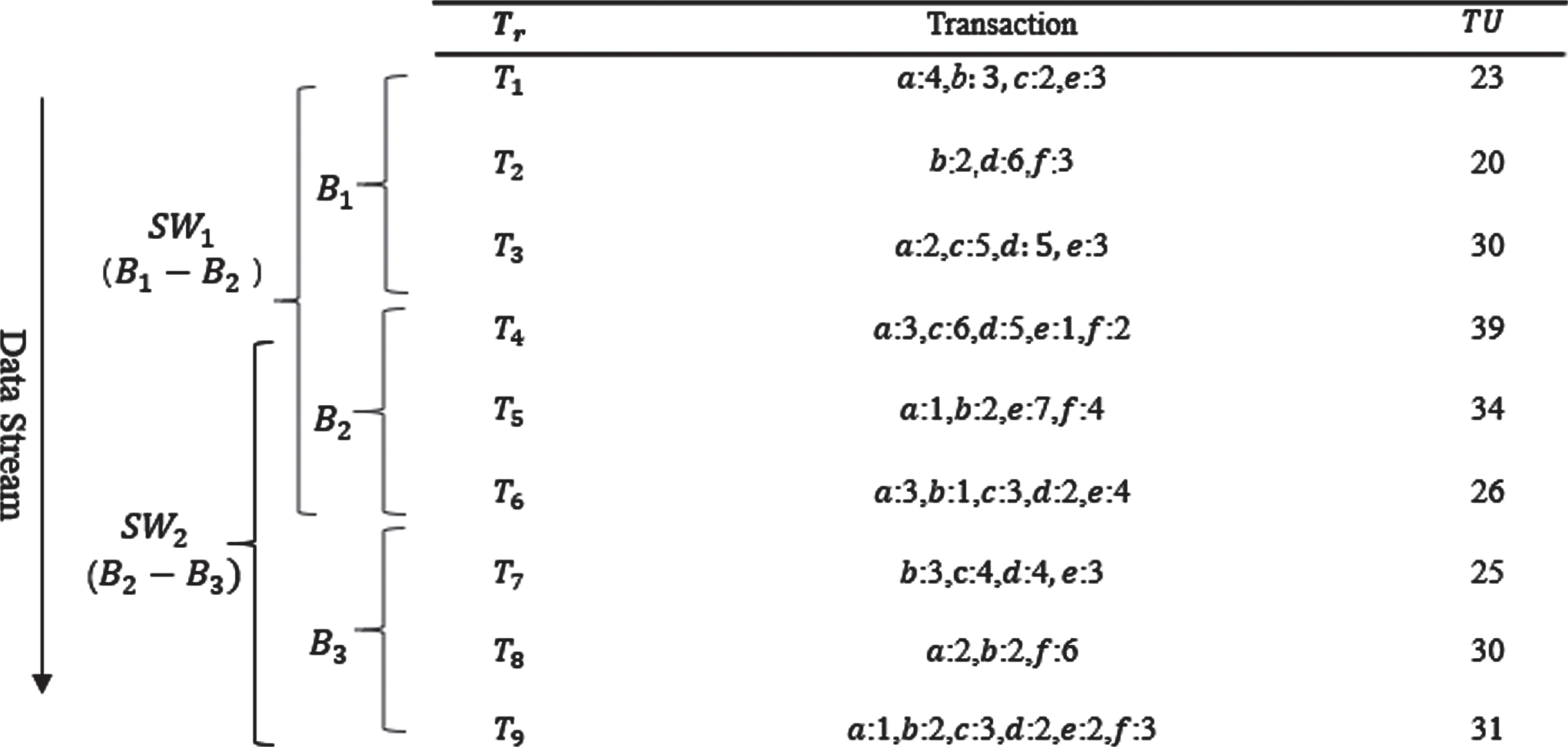
Example of a data stream.

Table 1

Profit table

Item	a	b	c	d	e	f
Utility	2	1	3	1	2	4

Definition 1 (Utility of an item) The utility of an item I_i(I_i ∈ I^*) in the transaction T_r is expressed as U (I_i, T_r), and defined as p (I_i, DS) × q (I_i, T_r). In a batch B, U (I_i, B) = ∑_{T_r∈_B}U (I_i, T_r). In a window SW_c, U_{SW
_c} (I_i) = ∑_{B∈SW_c}U (I_i, B).

Definition 2 (Utility of an itemset) The utility of an k-itemset X ={ I₁, I₂, …, I_k } in transaction T_r is expressed as U (X, T_r) and defined as $\sum_{I_{\dot{i}} \in X} U (I_{\dot{i}}, T_{r})$ . In a batch B, U (X, B) = ∑_{T_r∈_B}U (X, T_r). In a window SW_c, U_{SW
_c} (X) = ∑_{B∈SW_c}U (X, B).

Definition 3 (Transaction utility (TU)) The transaction utility of transaction T_r is expressed as TU (T_r) and defined as ∑_{∀I_i∈T_r}U (I_i, T_r). For example, the transaction utility of T₁ is TU (T₁) = U ({ ABCE } , T₁) , TU (T₁) = 23.

Definition 4 (High-utility itemset (HUI)) If the utility U_{SW
_c} (X) of an itemset X in the window SW_k is no less than minutil, then X is a high-utility itemset in SW_c. For example, the utility of {be} in window SW₁ is U_{SW
_c} ({ be }) = U ({ be } B₁) + U ({ be } B₂) = 9 +25 = 34.

Definition 5 (Transaction-weighted Utilization (TWU)) The TWU of an itemset X is the sum of the transaction utility of all transactions containing X in the current window SW_c. It is expressed as TWU (X) and defined as ∑_{X⊆T_r∩T_r∈SW_c}TU (T_r).

E.g, in the sliding window SW₁, TWU ({ ac }) = TU (T₁) + TU (T₃) + TU (T₄) + TU (T₆) = 23 + 30 + 39 + 26 = 118.

Definition 6 ((High Transaction-weighted Utilization Itemset in the window) If TWU (X) is no less than minutil, then the itemset X is a high transaction-weighted utilization itemset in window SW_c.

Property 1 ^[1](Pruning search space using TWU) Suppose there is an itemset X that is not a high TWU itemset, then X and its superset are both low-utility itemsets.

Definition 7 (Remaining utility) Let I_{SW
_c} be a set of items from I^*, ≻be an ordering on items from I_{SW
_c}, and X be an itemset. The Remaining utility of X in a transaction T_r is defined as Re (X, T_r) = ∑_{z∈T_r∧z≻y∀y∈X}U (z, T_r). The remaining utility of an itemset X in window SW_c is defined as Re_{SW
_c} (X) = ∑_{T_r∈g(X)∧T_r∈SW_c}Re (X, T_r) where g (X) is the set of transactions containing X.

Definition 8 (Remaining utility upper-bound) Let X be an itemset, and let the extensions of X be the itemsets that can be obtained by appending an item z to X such that z ≻ y, ∀y ∈ X. The remaining utility upper-bound of X in window SW_c is defined as Reu_{SW
_c} (X) = U_{SW
_c} (X) + Re_{SW
_c} (X).

Definition 9 (Extension upper-bound) Let X be an itemset. The extension upper-bound of itemset X in window SW_c can be defined as extUB_{SW
_c} (X) = ∑_{T_r∈C(X)∧T_r∈SW_c}U (X, T_r) + Re (X, T_r), where C (X) is the set of transactions containing X with re (X, T_r) > 0.

Property 2 (Abandoning extension based on extension upper-bound) If extUB_{SW
_c} (X) < minUtil, all extensions of X are low-utility itemsets and we do not need to extend the itemset X further.

Problem statement For each sliding window over the data stream, the task of Top-K high-utility itemset mining is to find the K HUIs with the largest utility in each window, where K is a user-defined parameter.

4 Proposed method

In this section, we analyze the key technologies of the proposed algorithm called ETKDS step by step. Subsection 4.1 describes a new simplified data structure designed by ETKDS to store the information of items. Subsection 4.2 introduces the construction method of the search space of ETKDS and related technologies to make the dataset scanning efficient. Subsection 4.3 introduces the mechanism proposed by ETKDS to maintain the efficiency and correctness of the projection in the current search space. Subsection 4.4 introduces multiple threshold raising technologies and a storage structure designed to cooperate with these technologies. Subsection 4.5 describes the main procedures and execution process of ETKDS.

4.1 CIUDataListSW structure

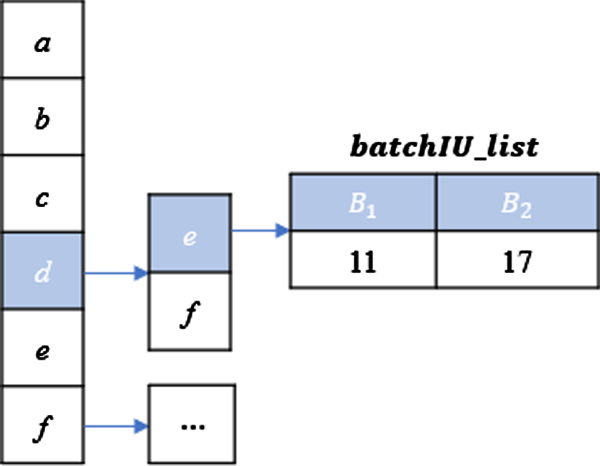
CIUDataListSW is a list of nodes containing key information from the current sliding window U_{SW
_c}. Each node is used to store the information of the item in the current sliding window and maintain transactions related to the item in batches. Figure 2 shows the structure of a node of CIUDataListSW that has the following fields:

Item: Information about the item represented by this node.

Utility: According to Definition 1, the utility U_{SW
_c} of the item in the current sliding window SW_c.

ExtUB: According to Definition 9, the extension upper-bound of the item in the current sliding window.

BatchData_List: the list of BatchData.

Fig. 2

Structure of a node of CIUDataListSW.

The detailed information and functions of the structure are as follows:

The utility of the item is used to determine whether the item is a HUI of length 1. extUB_{SW
_c} is used to determine whether to extend this item. If extUB_{SW
_c} is less than minutil, the longer itemset starting from this item will not be searched. BatchData includes BatchNumber, TransProjection, BatchTWU. TransProjection represents the transaction pseudo-projection of the current item in the batch numbered BatchNumber. Each record in TransProjection contains: the Tid of the transaction, the offset of the item in the sorted transaction, the utility of the item in the transaction, and TU of the transaction. BatchTWU records the TWU of each batch of items. BatchData_List can be directly used to construct the initial projected dataset of the item. In summary, the CIUDataListSW structure provides convenience for the subsequent sub-projection of itemsets through the stored projected dataset sorted in ascending order of TWU, and TWU, U_{SW
_c} and extUB_{SW
_c} can be updated quickly when batches are added or deleted.

Compared with the iList structure proposed by the Vert_top-k DS algorithm, CIUDataListSW is only used to store the transaction and utility information of items of length 1. You can use the TransProjection in the structure to directly create the dataset of the sub-projection to mine the subsequent extensible itemsets. Finally, the HUIs is obtained, and the subsequent process will not create any new structures. Compared with the traditional static Top-K high utility itemset mining algorithm TKEH 0, construction method and construction time of CIUDataListSW are different from TKEH. The algorithm ETKDS directly constructs its projection structure for each item during the second scan of the dataset, which means ETKDS has completed the construction of pseudo projections of all items at the end of the second dataset scan. TKEH first constructs the utility array for the entire reorganized dataset, and then constructs its local projection for each item. That is to say, TKEH needs to research arrays storing the original dataset to construct projection arrays for all items in turn after two dataset scans. Assuming that there is a fairly dense dataset (m rows and n items), this process will need n additional global dataset scans, and the time complexity of this process is about O (nmlogn). Therefore, this paper has obvious advantages in dataset scanning and the data structure. Compared with the nodes of IUDataListSW proposed by SOHUPDS [18], the node structure of CIUDataListSW is more concise. The node in IUDataListSW sets up identification fields for batch insertion and deletion, but the high-utility pattern update strategy using these fields is not friendly to dense datasets for the reason that items may be frequently inserted and deleted with batch updating. SOHUPDS needs to delete the Trie-tree associated with this node, and creates a new Trie-tree associated with this node. Therefore, the cost of time and space is extremely high. CIUDataListSW makes up for the shortcomings of the former and improves the performance of the algorithm on dense datasets. In addition, the structure of the node in CIUDataListSW adds the field BatchTWU, which allows the algorithm to efficiently update the TWU of the item after the sliding window changes which can save calculation time.

4.2 Scanning the dataset efficiently

This subsection mainly introduces the construction mechanism of the search space and related technology of efficiently scanning datasets in the algorithm proposed in this paper. In order to reduce the search space of the algorithm [3 , 6], the algorithm uses the best search space for all sliding windows, which is described in Subsection 4.2 (1). In order to reduce the cost of dataset scanning, ETKDS adopts dataset projection and projected transaction merging technologies, which are described in Subsection 4.2 (2) and (3) respectively. And in Subsection 4.3, the mechanism proposed by the algorithm to maintain the efficiency and correctness of the projection in the current search space is introduced.

(1) Search space in each sliding window

I_{SW
_c} is the set of items in the current window SW_c, let ≻ be a total order of items from I_{SW
_c}. According to this order, the search space of all itemsets 2^{I
_{SW
_c}} can be represented as a set-enumeration tree. The ETKDS algorithm executes a depth-first search from the root (empty set) until it explores the entire set-enumeration tree. For any itemset X during the depth-first search process, ETKDS will recursively append one item at a time to X according to the total order to generate a larger itemset. In the implementation of the search space in the current sliding window in this paper, ≻ is defined as the ascending order of the TWU of the items in I_{SW
_c}, for it usually reduces the search space of HUIM [2 , 10].

At present, the most advanced high-utility itemset mining algorithm from a data stream under sliding window model, SOHUPDS, uses lexicographic order to sort items and constructs a search space. Vert_top-k DS [16], the most advanced algorithm for mining Top-K high-utility itemsets from data streams singly uses TWU ascending order for the first window, and the order of the next window is fixed. The TWU ascending order is considered the best order. Especially in a data stream environment, data usually drifts over time. The use of a completely constant search space for each sliding window may greatly increase the unnecessary search process. Therefore, the dynamic search space proposed in this paper for each sliding window has certain environmental adaptability to ensure that the algorithm has good and stable mining efficiency in each sliding window.

Definition 10 (Item that can extend an itemset in the current window SW_c)

Let X be an itemset. E (X) is the set of items that can be used to extend X in the window SW_c according to the ordering, i.e., E (X) = {z|z ∈ I_{SW
_c} ∧ z ≻ x, ∀ x ∈ X}.

For example, consider the database of our running example and X ={ d }. The set E (X) is {e, f} if the ordering is set as the lexicographic ordering.

Definition 11 (Local utility)

Let X be an itemset and an item z ∈ E (X). The local utility of z w.r.t. X in woindow SW_c is lu_{SW
_c} (X, z) = ∑_{T_r∈g(X∪{z})∧T_r∈SW_c} [U (X, T_r) + Re (X, T_r)].

Property 3 (Pruning an item from all sub-trees using the local utility)

Let X be an itemset and an item z ∈ E (X). If lu_{SW
_c} (X, z) < minUtil, all extensions containing z are low-utility itemsets in SW_c. In other words, item z can be ignored when exploring all sub-trees of X, i.e., all extensions of X in the depth first search [12].

Definition 12 (Primary and Secondary items)

Let X be an itemset. In the window SW_c, the primary items of X is the set of items defined as Primary (X) = {z|z ∈ E (X) ∧ extUB_{SW
_c} (X ∪ z) ⩾ minUtil}. The secondary items of X is the set of items defined as Secondary (X) = {z|z ∈ E (X) ∧ lu_{SW
_c} (X, z) ⩾ minUtil}. Because lu_{SW
_c} (X, z) ⩾ Reu_{SW
_c} (X ∪ z) ⩾ extUB_{SW
_c} (X ∪ z), Primary (X) ⊆ Secondary (X).

(2) Dataset scanning using projection

The proposed algorithm calculates the utility and upper-bound values of the itemset by scanning the dataset. Since the dataset may be very large, it is very important to control the cost of dataset scans. Effectively reducing the size of the dataset is an urgent issue that HUIM needs to consider. When considering the itemset α in the depth-first search process, the algorithm needs to scan the database to calculate the utility and upper-bound values of itemsets in the subtree or the higher subtree of X. At this time, there is no need to scan those items that do not exist in E (X). A dataset composed of transactions without these items is called a projected dataset.

In order to efficiently implement dataset projection, ETKDS sorts each transaction according to the total order ≻ of the current sliding window SW_c. After the original transaction sorting is completed, the pseudo-projection is started, that is, each projected transaction is represented by the offset of the item or itemset in the corresponding original transaction. The pseudo-projection of a single item is exclusively maintained using the CIUDataListSW structure. As mentioned earlier, the value of the offset is represented by offset.

Definition 13 (Projected dataset) The projection of a transaction T using an itemset X is denoted as X - T, and defined as X - T = {i|i ∈ T ∧ i ∈ E (X). The projection of a dataset D using an itemset X is denoted as X - D, and defined as X - D = {X - T|T ∈ D ∧ X - T = ∅}.

(3) Dataset scanning using projected transaction merging

After performing the dataset projection, there exists many same transactions. The projected transaction merging technology can further reduce the cost of the algorithm to perform dataset scanning. SOHUPDS [18] also used dataset projection technology, but it did not adopt some effective strategies to merge the same transactions. Considering that the transactions over data streams have the characteristics of massiveness, the number of the same transactions is usually huge. Applying the projected transaction merging technology on the projected dataset can greatly reduce the size of the dataset. Therefore, it is very necessary to perform the projected transaction merging technology in the process of dataset projection.

Definition 14 (Projected transaction merging)

Replace a set of identical transactions T_{r
₁}, T_{r
₂}, …, T_{r
_m} in dataset X - D with a new transaction T_m, where the internal utility of each item in transaction T_m is defined as q (i, T_M) = ∑_k=1…mq (i, T_{r
_k}) .

The main problem in implementing this technique is to identify the same transactions. For this reason, this paper needs to compare all projected transactions with each other. In order to effectively implement this technique, the algorithm has pre-sorted all transactions according to the total order ≻ of the current sliding window before creating the projected dataset using the expandable item, ensuring that all the same transactions are found in O (n) time.

4.3 Reorganization technology for projected transactions in common batches

When the previous sliding window SW_c-1 is updated to window SW_c, the set of items in the sliding window I_{SW
_c-1} is updated to set I_{SW
_c}. The ascending order of the TWU generated in the previous window SW_c-1 and TWU of items will also change in this situation. The order before the change is denoted as ≻_c-1. Therefore, items will be reordered in the ascending order of TWU for the newly created window SW_c after the arrival of the new batch, and the new order is denoted as ≻_c. According to the projection mechanism described in Subsection 4.2 (2), the algorithm needs to sort the transactions in the new batch in order ≻_c. This brings about a new problem, that is, the sort order ≻_c-1 used by the transactions inherited from the previous window (the transactions in common batches) is out of date, and the sort order of the transactions in common batches is inconsistent with the transactions in the new batch. In order to maintain the spatial advantage of the search space of the algorithm (described in Subsection 4.2 (1)) and the execution efficiency of dataset projection, and ensure the accuracy of the projection (described in Subsection 4.2 (2)), designed a reorganization technology for projected transactions in common batches. This technology uses the order ≻_c to reorder CIUDataListSW’s projected transactions inherited from the previous window SW_c-1, that is, the transactions contained in common batches are effectively reorganized according to the order ≻_c, so that these transactions and the transactions in the new batch are kept in the latest order.

As described in Subsection 4.1, the item records its position in the projected transaction through the variable offset. The key to reorganization is to update the offset of the projections in all common batches according to the order of the new sliding window.

When a new batch arrives, a new window SW_c is created. When the algorithm scans the dataset for the first time, first it will record all items contained in SW_c, and the set of items is denoted as I_{SW
_c}. At the same time, the TWU of items is updated to obtain a new ascending order ≻_c, and construct a new search space. It traverses items in the set I_{SW
_c} in turn when the algorithm scans the dataset for the second time, and processes the transactions in common batches of the node of CIUDataListSW associated with each item. First, reorder the items in each transaction in order ≻_c. Since the transaction projection is a pseudo-projection, this means that the projected transactions with the same Tid in all nodes of CIUDataListSW are linked to the same memory address. Therefore, projected transactions with the same Tid in other nodes of CIUDataListSW do not need to be sorted again after sorting a certain projected transaction containing a certain item.

Subsequently, the algorithm searches each sorted projected transaction item by item until the current traverse item is found, and gets the position of the current traverse item in each reorganized transaction. The algorithm uses the position value to update the offset or other information of the projected transaction. The method process is shown in Algorithm 1.

Algorithm 1 Reorganization of projected transactions contained in common batches
Input:I_{SW _c}: a set of items in window SW_c, CIUDataListSW: a list of nodes containing the information from the current window SW_c, ≻_c: total order in the current window SW_c.
Output:CIUDataListSW: The list of nodes that have been reorganized.
1 For each item i in I_{SW _c}
2 If TWU (i) ⩾ minutil
3 Itemnode = CIUDataListSW.getNode(i);
4 For each transaction T in Itemnode.BatchData(all common batches)
5 If T is visited for the first time
6 Reorder T according to ≻_c
7 Find new offset of item i in transaction T after reorder
8 Update the projected transaction information of the Itemnode
9 Return CIUDataListSW

4.4 Threshold raising strategies

This paper uses CUD, CUDCB strategies and the actual utility of the 2-itemset stored in the CUDH _ SW structure to raise the minutil. Threshold raising strategies should be efficient in terms of execution time and memory usage, so the two strategies share the same structure to help achieve the above goals.

4.4.1 CUDH _ SW structure

A previous work 0 proposed to use the utility of 2-itemsets stored in the CUDM to raise the minutil. One of these itemsets may be a high utility itemset because the CUDM contains the utility of all 2-itemsets whose TWU is no less than minutil. But the TWU of items will be updated frequently, and the utility of 2-itemsets will also change frequently under the sliding window model as the window slides. It is necessary for the CUDM to recalculate the utility of 2-itemsets in each batch every time a sliding window is created because it can not save data in historical batches. Therefore, the CUDM is no longer suitable for the sliding window model. In order to solve this problem, this paper designs a new structure called CUDH _ SW. The CUDH _ SW is a double-layer hash table in the form of 〈I₁, 〈 I₂, batchIU_list 〉〉. The batchIU_list is a list composed of the utility of {I₁I₂} in each batch in the current window SW_c. Each record in the batchIU_list contains the batch name B and the utility of {I₁I₂} in batch B. For example, 〈d, 〈 e, batchIU_list 〉〉 represents the batchIU_list of itemset {de}. For a 2-itemset {I₁I₂}, the algorithm inserts {I₁I₂} into the CUDH _ SW if TWU ({ I₁I₂ }) > 0. Figure 3 is a schematic diagram of the CUDH _ SW in window SW₁ in the example in Chapter 3, and takes the itemset {de} as an example to show the utility stored in CUDH _ SW.

Fig. 3

CUDH _ SW of itemset {de} in window SW₁.

Definition 15 (common batches) SW_c-1 ={ B_j-1, B_j, …, B_n-1 } , SW_c = { B_j, B_j+1, …, B_n }, The common batches of SW_c-1 and SW_c are defined as CommonBatches ={ B_j, B_j+1, …, B_n-1 }.

$\begin{matrix} \forall X \subseteq T_{r} \land T_{r} \in B \land B \in CommonBatches, U_{{SW}_{c - 1}} (X) \\ = \sum_{l = j - 1}^{n - 1} U (X, B_{l}) \\ = \sum_{B \in CommonBatches} U (X, B) + U (X, B_{j - 1}), U_{{SW}_{c}} (X) \\ = \sum_{l = j}^{n} U (X, B_{l}) = \sum_{B \in CommonBatches} U (X, B) + U (X, B_{n}) \end{matrix}$ (1)

According to Definition 15, calculating the actual utility of itemset {I₁I₂} in windows SW_c-1 and SW_c respectively involves calculating the utility of {I₁I₂} in CommonBatches. The utility of any batch in CommonBatches can be reused in the construction of CUDH _ SW in the next sliding window. Obviously, this structure eliminates the need for the algorithm to recalculate the utility of 2-itemsets that meet the conditions in each common batch, so as to shorten the time of the threshold raising strategy in the preparation phase. The working mechanism of batch deletion and insertion in the batchIU_list maintained by CUDH _ SW will be further introduced in Subsection 4.5.

4.4.2 CUD(Cooccurrence Utility decreasing order)

According to Definition 15 and the batchIU_list of all 2-itemsets in the CUDH _ SW, the approach calculates the utility of these itemsets in the current sliding window SW_c, and adds these utilities to a priority queue CUQ in descending order. Suppose the total number of utility values added to the CUQ is N, and the number of HUIs set by the user is K. According to Property 4, the value in the CUQ at the index of K (K ⩽ N) can be set as the candidate minimum utility threshold, denoted as $\underset{c}{minutil} {andit}_{C} UD$ . Once $\underset{c}{minutil} {andit}_{C} UD$ is greater than the previous minimum utility threshold, $\underset{c}{minutil} {andit}_{C} UD$ will become the new minutil. The method process is shown in Algorithm 2.

Property 4 Let H_{SW
_c} denote the Top-K high utility itemsets in the window SW_c. Let K_CUD_{SW
_c} be the K-th largest utility in the CUQ. We have that U_{SW
_c} (X) ⩾ K_CUD_{SW
_c}, ∀X ∈ H_{SW
_c.}

Proof. Let CUDH _ SW_K ={ X ∈ CUDH _ SW, U_{SW
_c} (X) ⩾ K_CUD_{SW
_c} }. Assume that ∃Y ∈ H_{SW
_c}, U_{SW
_c} (Y) < K_CUD_{SW
_c}. We have that ∀X ∈ CUDH _ SW_K, U_{SW
_c} (X) ⩾ K_CUD_{SW
_c} > U_{SW
_c} (Y). Therefore, CUDH _ SW_K ⊆ H_{SW
_c}. Furthermore, Y ∈ H_{SW
_c}. This is in contradiction with the statement that H_{SW
_c} is the set of Top-K high utility itemsets. Thus, ∄Y ∈ H_{SW
_c}, U_{SW
_c} (Y) < K_CUD_{SW
_c}, which means that U_{SW
_c} (X) ⩾ K_CUD_{SW
_c}, ∀ X ∈ H_{SW
_c}.

Algorithm 2 CUD Strategy
Input:K: desired number of HUIs, CUDH _ SW: a structure to store the utility of 2-itemsets
Output:minutil .
1 Calculate the utility of 2-itemsets in the current window SW_c used the CUDH _ SW structure
2 Put these utilities into a decreasing priority queue called CUQ
3 Save the utility of 2-itemsets in common batches into the Cache When running the first line of
code
4 $\underset{c}{minutil} {andit}_{C} UD = CUQ [K]$
5 $minutil = max {minutil, \underset{c}{minutil} {andit}_{C} UD}$
6 Return minutil .

4.4.3 CUDCB

In order to provide a better initial threshold for the next sliding window SW_c+1, this paper designs a new threshold raising strategy called CUDCB. Under the sliding window model, the last {winSize - 1} batches remain unchanged between two consecutive windows (such as SW_c, SW_c+1), i.e. CommonBatches hereinbefore defined. Based on the above principles, the algorithm uses the information in the CUDH _ SW to calculate the utility of all 2-itemsets in the last {winSize - 1} batches of the current sliding window SW_c. Similar to the procedure in CUD, these values are added to a priority queue called CUCBQ, and the new minutil is obtained by index K.

Different from the CUD strategy, the value indexed in the CUCBQ is directly used as the initial minutil of the next sliding window SW_c+1. A more suitable initial threshold will greatly reduce the search space of the algorithm. Since the next sliding window contains the new batch of transactions, the utility of the 2-itemset in SW_c+1 can only be greater than or equal to its utility in the current common batches of SW_c and SW_c+1. What’s more, we know that this strategy can still make algorithm generate at least K HUIs according to Property 5. The strategy process is shown in Algorithm 3.

Property 5 Let H_{SW
_c+1} denote the Top-K high utility itemsets in the window SW_c+1. Let K_CUDCB_{SW
_c} be the K-th largest utility in the CUCBQ of SW_c. We have that U_{SW
_c+1} (X) ⩾ K_CUDCB_{SW
_c}, ∀ X ∈ H_{SW
_c+1}.

Proof. Hence K_CUDCB_{SW
_c} = K_CUDCB_{SW
_c+1} ⩽ K_CUD_{SW
_c+1}, and U_{SW
_c+1} (X) ⩾ K_CUD_{SW
_c+1}, ∀ X ∈ H_{SW
_c+1}. Therefore, U_{SW
_c+1} (X) ⩾ K_CUDCB_{SW
_c+1} = K_CUDCB_{SW
_c}, ∀ X ∈ H_{SW
_c+1}.

The strategy adopted by the previous algorithm [16] needs to calculate the utility in common batches for all intermediate itemsets. The strategy proposed in this paper only needs to calculate and store the utility of 2-itemsets, thus reducing the computational time and memory overhead of the algorithm. At the same time, the utility calculation process of 2-itemsets in common batches is a subset of its utility calculation process in the entire sliding window, so this strategy does not need additional calculations, and the required values have been calculated and cached in advance when the CUD strategy is running. In summary, the biggest advantage of the CUDCB strategy is that it can quickly provide a higher initial minutil for the next sliding window without performing any additional calculations about utility with the help of the CUDH _ SW and the CUD strategy.

Algorithm 3 CUDCB Strategy
Input:Cache: a cache storing the utility of 2-itemsets in common batches of SW_c and SW_c+1, K: desired number of HUIs.
Output:minutil.
1 Extract the utility of 2-itemsets on common batches from Cache
2 Put these utilities into a decreasing priority queue called CUCBQ
3 minutil = CUCBQ [K]
4 Return minutil

4.5 ETKDS algorithm

In this subsection, this paper describes the ETKDS algorithm for mining Top-K high-utility itemsets under sliding window model. ETKDS utilizes several technologies or methods explained previously, including the CIUDataListSW structure, a reorganization technology for projected transactions in common batches, and some efficient threshold raising strategies, etc. In order to further improve the efficiency of dataset scanning and reduce the search space, ETKDS uses projected transaction merging technology, and uses a set enumeration tree composed of items sorted in increasing order of TWU as its search space in any sliding window. The main process of ETKDS is shown in Algorithm 4. First, ETKDS scans transactions over the data stream, and adds transactions to the current sliding window in batches (line 7). Window size and batch size depend on windowSize and batchSize respectively. At the same time, the old batch will be deleted as the sliding window moves forward. ETKDS maintains and updates the CIUDataListSW and CUDH _ SW structures in the current sliding window by deleting the old batch and inserting the new batch (lines 10 to 17). When transactions in the old batch is deleted, TWU needs to subtract the BatchTWU of the old batch. The utility record of the old batch in the batchIU_list of the CUDH _ SW of 2-itemsets are also deleted at the same time. When a new batch is inserted, the information about the new batch in the CIUDataListSW and CUDH _ SW structures will be created. Sort all items I_{SW
_c} in the current sliding window SW_c in ascending order of TWU, and then denote the order by ≻_c. When scanning the dataset for the second time, the algorithm sorts the items in the transaction according to ≻_c (line 19), and this sort is used as the total order of the remaining steps of the algorithm (line 22). If the current window is not the first window generated by the algorithm, the transactions in these batches are sorted according to the order ≻_c-1 of the previous window SW_c-1 because common batches of the current window is retained from the previous window. As described in Subsection 4.3, the algorithm needs to reorganize the projected transactions in common batches in the order ≻_c of the current window, and it also needs to update the extUB_{SW
_c} and offset of the node of CIUDataListSW, to prepare for the next mining process (line 21).

Before starting the mining process, the initial minutil of the first created window is set to 0. The algorithm inserts each item and its utility into a Top-K priority queue named KQ, and then sorts utilities in the KQ in descending order (lines 23 to 26). ETKDS compares the K^th utility value in the KQ with the current minutil, and the larger value is used as the new minutil (line 27). It is worth noting that, except for the initial minutil of the first sliding window, which is initially 0, the initial minutil of remaining windows is given by the CUDCB strategy. According to Property 1, items of TWU < minUtil and their supersets will not be HUIs. Therefore, items with TWU ⩾ minutil are added to a set of items Secondary (∅) (line 28). As a set of promising items, Secondary (∅) will be used to construct the search space. The algorithm calls the CUD strategy and updates the minutil (line 29). Then the algorithm calculates extUB_{SW
_c}for each item in the set Secondary (∅). According to attribute 2, any extension under the subtree of item i will not become a HUI if extUB_{SW
_c} (i) is less than minutil. Therefore, ETKDS will add the item i to the set Primary (∅) if extUB_{SW
_c} (i) is no less than the current minutil (line 30). Then ETKDS traverses the item i in the set Primary (∅), and searches supersets at the beginning of i. Since theCIUDataListSW records the Tid of transactions and the offset of the item in transactions, the process can directly use the above information to create the projected dataset γ - DB of item i without rescanning the original dataset. Later, ETKDS needs to consider promising items that can be used to extend i. First, the algorithm creates a set of candidates called sItems (line 33). Then, the algorithm calculates extUB_{SW
_c} (γ ∪ z) andlu_{SW
_c} (γ, z) for each item z ∈ sItems, and generates sets Primary (γ) and Secondary (γ) by scanning the projected dataset γ - DB once which are used to call the procedure Search to start mining the extended itemset of γ (lines 34 to 36).

The Search procedure (algorithm 5) takes six input parameters: an item γ, which needs to be extended for longer itemsets, the projected datasetγ - DB, which generated by projected transactions in the node for item γ in the CIUDataListSW, Primary (γ), Secondary (γ), minutil and a priority queue KQ. The procedure creates an extended itemset β ={ γ ∪ x } for each item x ∈ Primary (γ), and then generates β - DB using projected transaction merging, which is the projected dataset of β from γ - DB(lines 1 to 3). The procedure checks whether the itemset β is a HUI. The algorithm will insert β into the priority queue KQ, and update minutil if the actual utility of β is no less than the current minutil (lines 4 to 5). The procedure scanning β - DB, similar to Algorithm 4, still needs to filter out candidate items from the set Secondary (γ) and put them into the set sItems (line 6). Then extUB_{SW
_c} (β ∪ z) and lu_{SW
_c} (β, z) are calculated for each itemz ∈ sItems (line 7). According to the above utility information, Property 3 and Definition 12, The procedure finds two sets of items Primary (β) and Secondary (β) for the itemset β (lines 8 to 9). Then the Searchprocedure is called recursively to extend the itemset β (line 10). In the above mining process, the algorithm uses the pruning strategy based on the lu utility to select the promising candidate extension items of β. Then, the algorithm uses the pruning strategy based on the extUB utility and the pruning strategy based on the lu utility to select the extendable son nodes of β and the promising candidate extension items of all the subtrees of β respectively from the previously selected promising candidate extension items of β to continue the recursive search. In other words, the pruning strategy based on the lu utility can significantly reduce the number of candidates calculated by the pruning strategy based on the extUB utility, and accelerate the efficiency of pruning process. Therefore, When the amount of data over data streams is large, it is beneficial to use two pruning strategies together.

After ETKDS completes the Search procedure of all items in the Primary (∅), ETKDS calls the CUDCB strategy to provide a initial minutil for the next sliding window (line 37). The threshold raising strategy CUDCB proposed in this paper is different from the Vert_top-k DS’s strategy adopted between sliding windows. There is no need for CUDCB to calculate and maintain the actual utility of all HUIs in each batch. As described in Subsection 4.4.3, this strategy is executed after the CUD and does not produce any calculation process about the utility value of the itemsets. Later, ETKDS returns the complete set of Top-K high-utility itemsets in the current sliding window (line 38). Then the sliding window continues to slide forward, and ETKDS starts the mining of Top-K high-utility itemsets in the subsequent sliding windows.

Algorithm 4 ETKDS
Input:DS: a data stream, batchSize: number of transactions in a batch, windowSize: number of batches in a sliding window, SW_c: currently created sliding window.
Output:KQ: a priority queue of size K containing Top-K high utility itemsets in the window SW_c.
1 Var currentBatch = 0
2 Var swTransDB;
3 While there is stream of transactions do
4 Init CUDH _ SW structure, Cache
5 Init priority queue CUQ, CUCBQ, a priority queue of size KKQ.
6 Var batchTransactions;
7 Read the transactions from data stream DS and add to batchTransactions according to batchSize;
8 ++currentBatch;
9 If currentBatch > windowSize then
10 Var oldBatchNumber = currentBatch - windowSize;
11 CIUDataListSW.removeOldData(oldBatchNumber);
12 swTransDB.remove(oldBatchNumber);
13 Update CIUDataListSW.TWU by
CIUDataListSW . TWU - CIUDataListSW.get(oldBatchNumber). BatchTWU
14 Remove CUDH _ SW . batchIU_list(oldBatchNumber)
15 swTransDB.add(batchTransactions);
16 CIUDataListSW.addBatchTransactions(batchTransactions)
17 Update CIUDataListSW . TWU and CUDH _ SW structure according to batchTransactions
18 If currentBatch ⩾ windowSize then
19 Let ≻_c be the total order of TWU ascending values on I_{SW _c}
20 If windowsNumber is not 1 then
21 Reorganization of projected transactions contained in common batches(I_{SW _c},
CIUDataListSW, ≻_c)
22 Sort the batchTransactions in currentBatch of SW_c according to ≻_c
23 For each item i in I_{SW _c}
24 Itemnode = CIUDataListSW.getNode(i);
25 If itemnode.Utility⩾minutil then
26 Insert (i, itemnode.Utility) into KQ
27 minutil = max {minutil, utility_kth_itemset}
28 Secondary (∅) = {i\|i ∈ I_{SW _c} ∧ TWU (i) ⩾ minutil} ;
29 CUD strategy(hashmap CUDH _ SW, K)
30 Primary (∅) = {i\|i ∈ Secondary (∅) ∧ extUB_{SW _c} (i) ⩾ minutil}
31 For item i inprimary (∅)
32 γ ={ i }
33 sItems = {j\|j ∈ Secondary (∅) ∧ j ≻ _ci}
34 Primary (γ) = {z\|z∈ sItems ∧ extUB_{SW _c} (γ ∪ z) ⩾ minUtil} ;
35 Secondary (γ) = {z\|z∈ sItems ∧ lu_{SW _c} (γ, z) ⩾ minUtil} ;
36 Search(γ,γ - DB, primary (γ), secondary (γ), minutil, KQ)
37 CUDCB strategy(Cache, K)
38 Return KQ
39 End while

Algorithm 5 Search
Input:γ : an itemset, γ - DB : a projected dataset, Primary (γ): the primary items of γ, Secondary (γ): secondary items of γ, minutil, KQ: a priority queue of K itemsets.
1 Foreach item x ∈primary (γ) do
2 β = γ∪ { x };
3 β - DB = β projected dataset from γ - DB using projected transaction merging;
4 If U_{SW _c} (β) ⩾ minUtil
5 Add β in KQ and raise the minutil to the top of priority queue element’s utility;
6 sItems = {j\|j∈ Secondary (γ) ∧ j ≻ _cx} ;
7 By scanning β - DB once, calculate U_{SW _c}(β ∪ z), extUB_{SW _c} (β ∪ z) and lu_{SW _c} (β, z), where
z ∈ sItems;
8 Primary (β) = {z\|z∈ sItems ∧ extUB_{SW _c} (β ∪ z) ⩾ minUtil} ;
9 Secondary (β) = {z\|z∈ sItems ∧ lu_{SW _c} (β, z) ⩾ minUtil} ;
10 Search(β, β - DB, Primary (β), Secondary (β), minUtil, KQ);

5 Experiments and results

In this section, we conducted experiments on a computer with 16 GB of available RAM, an Intel Core-i7-6700@2.60 GHz CPU, and running Windows 10 operating system. Compare the performance of our proposed algorithm ETKDS with the algorithm TKEH and Vert_top-k DS respectively, these algorithms are written in Java language. TKEH is currently the state-of-the-art algorithm for mining Top-K high-utility itemsets in static databases. Vert_top-k DS is the state-of-the-art algorithm for mining Top-K high-utility itemsets over data streams. In addition, this paper designs three variants of ETKDS in order to evaluate the impact of threshold raising strategies on ETKDS, which are called ETKDS(CUD), ETKDS(CUDCB), and ETKDS. Among them, ETKDS(CUD) is an algorithm that only uses the CUD strategy, ETKDS(CUDCB) is an algorithm that only uses the CUDCB strategy, and ETKDS simultaneously applies two threshold raising strategies. In Table 2, the datasets used in the comparison experiment with Vert_top-k DS are listed, and the batch size and window size are given, so that the two algorithms can run several batches on each dataset to evaluate the performance of algorithms in dynamic environment. Table 3 lists the dataset used in the comparison experiment with TKEH. Since TKEH is a static algorithm, it is different from the data environment in which our algorithm is designed to work. In order to control the experimental variables, our algorithm in this part of the experiment runs the whole dataset in a single window and single batch, and simulates mining in a static environment to evaluate the mining performance in a single window. Therefore, the window parameters of each dataset are not given in Table 3. Both tables describe the characteristics of the dataset, such as the number of transactions (#trans), the number of different items in the database (#items) and the average transaction length (#Avg. length). The ChainStore, Retail and Accidents, Chess, Foodmart and Mushroom datasets have real utility values. For other datasets, they have synthetic utility values, that is, the internal utility values have been generated using a uniform distribution in [1, 10]. ChainStore was obtained from the NUMineBench software distribution 1 , Connect was obtained from FiMi repository 2 , and other datasets was obtained from spmf 3 . The real size of Connect, ChainStore, Accidents, Chess, Foodmart, Mushroom, and Retail datasets are 16.1 MB, 79.2 MB, 63.1 MB, 641 KB, 175 KB, 1.03 MB, and 6.42 MB respectively. Experiments compare the algorithms on the following parameters: pattern results of mining, the total time required to mine Top-K high-utility itemsets, the average memory during operation, and the number of intermediate itemsets generated by some algorithms. Experiment in the following three situations: 1. Compare the change of K with TKEH and Vert_top-k DS. 2. Comparison against Vert_top-k DS for varying window size. 3. Comparison against Vert_top-k for different dataset size.

Table 2
The dataset used in the comparison experiment between our algorithm and Vert_top-k DS

Dataset #trans #Avg.length #items Type Window size Batch size

Connect 67557 43 129 Dense 3 10000

Retail 88162 10.3 16470 Sparse 3 10000

ChainStore 1112949 7.3 46086 Sparse 6 100000

Accidents 340183 33.8 468 Dense 3 50000

Dataset	#trans	#Avg.length	#items	Type	Window size	Batch size
Connect	67557	43	129	Dense	3	10000
Retail	88162	10.3	16470	Sparse	3	10000
ChainStore	1112949	7.3	46086	Sparse	6	100000
Accidents	340183	33.8	468	Dense	3	50000

Table 3

The dataset used in the comparison experiment between our algorithm and TKEH

Dataset	#trans	#items	#Avg.length	Type
Foodmart	4141	1559	4.42	Sparse
Retail	88162	16470	10.3	Sparse
Mushroom	8124	119	23	Dense
Chess	3196	75	37	Dense

5.1 Varying K

First, this paper compares the mining results with TKEH and Vert_top-k DS under the experimental dataset and its corresponding parameters. The comparison results are shown in Tables 4 and 5, respectively. The analysis result shows that when the Kvalue is the same, ETKDS and the static algorithm TKEH obtain the same K results when mining the same dataset. Under the same window size and batch size, our algorithm ETKDS finally generates exactly the same pattern results as Vert_top-k DS in all windows. In summary, it is proved that the results of our algorithm mining are complete and correct.

Table 4
Result evaluation between our algorithm and TKEH

Retail Mushroom Foodmart Chess

K Number (Patterns) consistency Number (Patterns) consistency Number (Patterns) consistency Number (Patterns) consistency

1 1 yes 1 yes 1 yes 1 yes

100 100 yes 100 yes 100 yes 100 yes

500 500 yes 500 yes 500 yes 500 yes

1000 1000 yes 1000 yes 1000 yes 1000 yes

Retail	Mushroom	Foodmart	Chess
1	1	yes	1	yes	1	yes	1	yes
100	100	yes	100	yes	100	yes	100	yes
500	500	yes	500	yes	500	yes	500	yes
1000	1000	yes	1000	yes	1000	yes	1000	yes

Table 5

Result evaluation between our algorithm and Vert_top-k DS

Connect		Retail		ChainStore		Accidents
K	Number (Patterns)	consistency	Number (Patterns)	consistency	Number (Patterns)	consistency	Number (Patterns)	consistency
1	5	yes	7	yes	7	yes	5	yes
100	500	yes	700	yes	700	yes	500	yes
300	1500	yes	2100	yes	2100	yes	1500	yes
500	2500	yes	3500	yes	3500	yes	2500	yes

Next, in order to verify the mining performance of our algorithm in a single window, ETKDS will be compared with the static algorithm TKEH. According to the experimental settings, ETKDS will construct a window with a batch size equal to the transaction size of the dataset and perform mining only once to ensure that the two algorithms have exactly the same input data. Because the CUDCB strategy has no practical meaning when used in a single window, this experiment uses ETKDS(CUD) instead of ETKDS to participate in the comparison. The experimental results of time evaluation are shown in Fig. 4.

Fig. 4

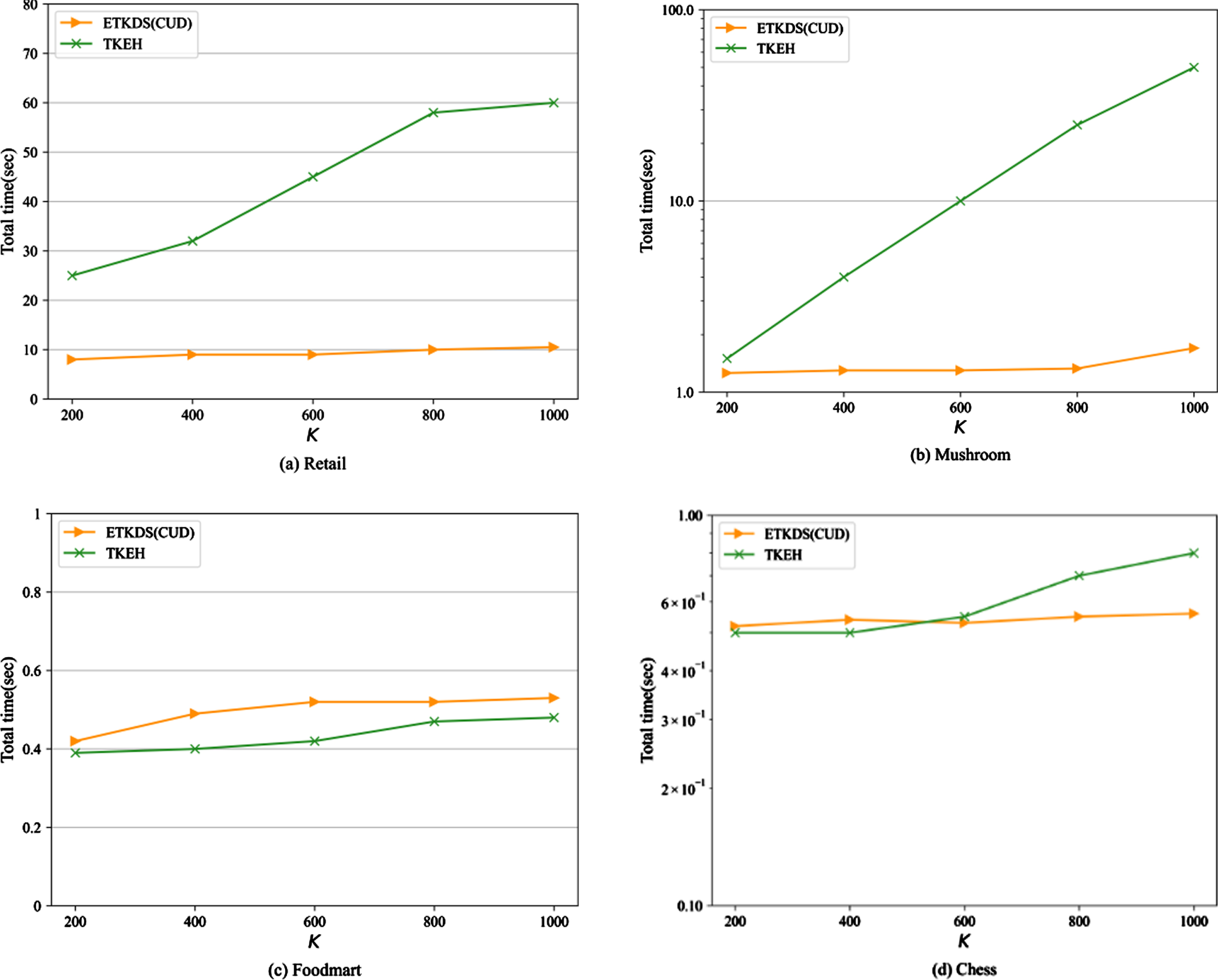
Effect of varying K in a single window on total running time.

By observing the experimental data, it can be seen that when the Kvalue is small, the algorithm often has a high initial minUtil. In this case, the biggest factor affecting the time performance of the algorithm is often the threshold raising strategy and the construction of data structure. Both algorithms use the RIU and CUD threshold raising strategy, and TKEH added COV threshold raising strategy additionally, it has been proved that COV has a good effect on sparse datasets such as Retail [13]. However, the time consumption of our algorithm on the Retail dataset is still less than that of TKEH, this is because the structure and structure construction method used in our algorithm have obvious advantages (as explained in Subsection 4.1). Therefore, when the number of items and transactions in the dataset is obviously large (for example, Retail), our algorithm will have a great speed advantage, while the transaction scanning speed of TKEH will be slow.

On datasets with small items and transactions, such as Chess, Mushroom, etc., in general, the algorithm ETKDS(CUD) obtains less time consumption when the K value is high. This is because the initial minUtil of the algorithm is low in this case, and both the pruning strategy and the threshold raising strategy have a great impact on the algorithm. By using local utility instead of TWU, ETKDS(CUD) can obtain a more compact upper limit of utility and further reduce the search space. The higher the K value, the more obvious the advantage of the search space pruning strategy.

Through memory experiment observation, our algorithm consumes less memory on datasets with fewer items such as Mushroom and Foodmart. When there are many items in a dataset, it will cost more memory. The reason is that our algorithm needs to establish a list structure for each item, which maintains the projection of different batches in the data stream, so this structure is more complicated than the array used by traditional static algorithms.

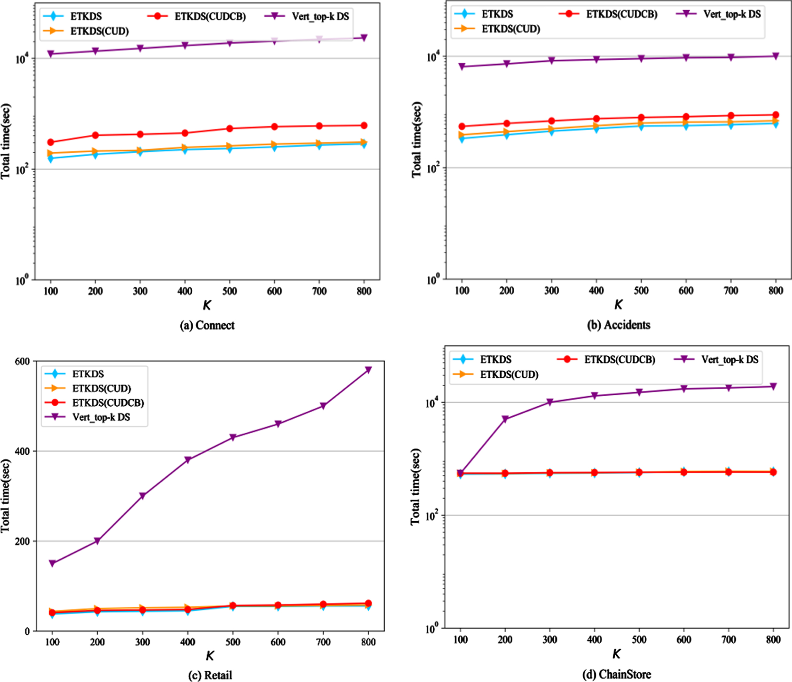
Then, this paper compares the performance of Vert_top-k DS and ETKDS proposed in this paper for various sparse and dense datasets. The parameter K varies between 100 and 800. The experimental results of running time are shown in Fig. 5, and the results of the number of intermediate itemsets generated are shown in Table 6. The results show that on almost all types of datasets, the running time of the proposed algorithm and its variants is lower than that of the comparison algorithm Vert_top-k DS, and the number of intermediate itemsets that need to be traversed is also less than Vert_top-k DS. However, the performance gap between algorithms is slightly different on different types of datasets.

Fig. 5

Effect of varying K in multiple windows on total running time.

Table 6

The number of intermediate itemsets generated by the algorithm for varying K

Dataset	K	ETKDS	ETKDS(CUD)	ETKDS(CUDCB)	Vert_top-k DS
Connect	100	964280	965076	1773701	15106166
	300	2359647	2359905	4215389	16714255
	500	4003832	4004060	6610411	20373328
	700	6031350	6031552	9456271	24765852
Accidents	100	146559	147445	237667	3462426
	300	457096	459134	747886	8285458
	500	613980	615870	2002543	8304026
	700	2702383	2714443	2745146	8504771
Retail	100	43445	44913	43708	24037137
	300	74818	77004	75839	98943831
	500	90877	93937	94166	156568444
	700	105545	110793	138390	222743759
Chain Store	100	40544	40544	40544	54957268
	300	119527	119527	119527	236253650
	500	154527	154936	154527	397792596
	700	181829	182080	181829	540608869

For dense datasets, ETKDS, ETKDS(CUB) use the K^th largest item’s utility to raise the minutil, and also use the K^th largest 2-itemset’s actual utility in the entire sliding window as the raised threshold, which is more useful than Vert_top-k DS using only the K^th largest item’s utility.

Specifically, ETKDS runs about 98 times faster than the comparison algorithm Vert_top-k DS on the Connect dataset, and the number of intermediate itemsets generated is reduced by an order of magnitude on average. On the Accidents dataset, the running time of ETKDS is about 90 ∼ 94 times faster than the comparison algorithm Vert_top-k DS at different K values, and the number of intermediate itemsets generated is also reduced by an order of magnitude on average. Although ETKDS(CUDCB) raises the threshold minutil less than ETKDS(CUD), and when the dataset is dense, the CUDCB may be slightly worse than the threshold raising strategy of Vert_top-k DS, because at this time, there are often high-utility itemsets with a length greater than 2. However, ETKDS(CUDCB) still has lower time consumption than Vert_top-k DS on all dense datasets, and generates fewer intermediate itemsets. This is because the algorithm proposed in this paper adopts the best search space construction method, uses the reorganization technology for projected transactions in common batches and more compact pruning strategies to greatly reduce the search space. At the same time, the projected transaction merging technology is used to merge the same transactions, which greatly reduces the number of scans of the dataset.

Comparing the experimental data of ETKDS and its variants on dense datasets, it can be found that the two threshold raising strategies used by ETKDS are effective. Compared with the ETKDS(CUD) and ETKDS(CUDCB) algorithms that use a single threshold raising strategy, ETKDS has the fastest execution time and the least number of intermediate itemsets, which shows that the two threshold raising strategies are effective on this type of datasets, because ETKDS has achieved better performance than ETKDS(CUD) and ETKDS(CUDCB) by using both CUD and CUDCU strategies. In addition, most items often appear evenly in all batches in dense datasets, but the CUDCB strategy only calculates the utility of 2-itemsets in common batches. Therefore, ETKDS and ETKDS(CUD) generate fewer intermediate itemsets than ETKDS(CUDCB) in most cases, and the running time is lower. On the Connect dataset, the candidate itemsets generated by ETKDS is about 35% -45% less than the ETKDS(CUDCB) that only uses the CUDCB strategy, and the running time is reduced by 52%. On the Accidents dataset, the candidate itemsets generated by ETKDS is reduced by about 45% at the maximum compared with the ETKDS(CUDCB) that only uses the CUDCB strategy, and the running time is reduced by about 31% on average.

For sparse datasets, the running times of ETKDS, ETKDS(CUDCB) and ETKDS(CUD) are very close. Although the CUD and CUDCB strategies reduce the number of intermediate itemsets to a certain extent (such as the Retail dataset in Table 6), the items in the dataset may only appear in very few transactions. With the deepening of the projection process, the number of projected transactions that need to be searched in the process of an itemset extension decreases rapidly, and the level of recursive projection of items is generally smaller than that on dense datasets. Therefore, the projection construction cost of the algorithm and the dataset scanning cost are greatly reduced, resulting in slight changes in the number of intermediate itemsets and different threshold raising strategies having very limited effects on saving the running time of the algorithm proposed in this paper. Experiments also show that the CUDCB strategy is not better than Vert_top-k DS on the basis of the threshold raising effect. ETKDS(CUDCB) can still maintain a large time advantage with the comparison algorithm Vert_top-k DS, which shows that ETKDS and its variants can guarantee a smaller search space on the basis of transaction reorganization. By further using the projection technology and multiple pruning strategies, ETKDS(CUDCB) prunes a large number of intermediate itemsets. Vert_top-k DS generates a large number of intermediate itemsets and requires a large number of vertical utility-list structure construction and join operations for the reason that its pruning strategy is not compact enough. In terms of intermediate itemsets, the number of intermediate itemsets generated by ETKDS(CUDCB) is about 3 orders of magnitude less than that generated by Vert_top-k DS on ChainStore and Retail datasets. In terms of running time, the running time of ETKDS(CUDCB) is reduced by about 93% and 70% respectively compared with Vert_top-k DS on the ChainStore and Retail datasets.

5.2 Varying window size

For the sliding window model, the window size has a great influence on the running effect of the model. In order to analyze the impact of this parameter, this subsection fixes K to 500, and uses the dense dataset Accidents and the sparse dataset ChainStore to conduct experiments under various parameters to evaluate the running time and memory consumption of the algorithm ETKDS. As is shown in Table 7 and Fig. 6, the number of intermediate itemsets generated by ETKDS decreases as the window size increases on the ChainStore dataset. On the Accidents dataset, the number of intermediate itemsets increases with the increase of window size. Due to the denseness of the Accidents dataset, a large number of long high-utility itemsets are often generated, and the cost of projection will gradually increase. Due to the characteristics of sparse datasets, opposite results appear on the two datasets. The changing trend of the running time is basically the same as that of the number of candidate itemsets, that is, the running time required for ETKDS on the Accidents dataset is increasing, while the running time required for ETKDS on the ChainStore dataset is decreasing. Compared with Vert_top-k DS, ETKDS has lower time consumption on both datasets, which shows that there is a certain correlation between the running time and the number of intermediate nodes actually traversed in the search space for the two algorithms.

Table 7
The number of intermediate itemsets generated by the algorithm for varying window size

Dataset Window size ETKDS Vert_top-k DS

Accidents 3 613980 6568143

4 734051 6531135

5 826609 6973685

6 856735 7249794

7 1120831 115764035

Chain Store 2 253259 233605737

4 196914 577255173

6 154527 497792596

8 111126 397792596

10 66193 297792596

Dataset	Window size	ETKDS	Vert_top-k DS
Accidents	3	613980	6568143
	4	734051	6531135
	5	826609	6973685
	6	856735	7249794
	7	1120831	115764035
Chain Store	2	253259	233605737
	4	196914	577255173
	6	154527	497792596
	8	111126	397792596
	10	66193	297792596

Fig. 6

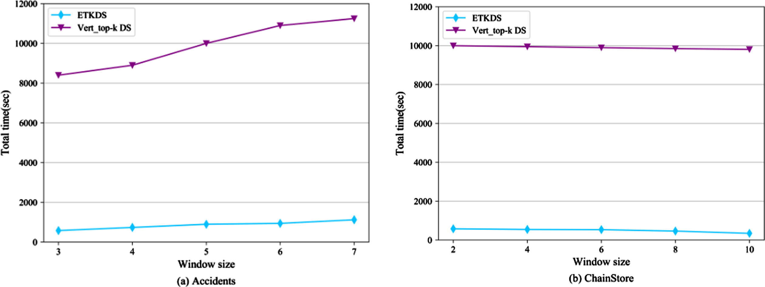
Effect of varying window size on total running time.

The more critical point is that the reorganization technology for projected transactions in common batches used by ETKDS enables each sliding window to have a smaller search space, and also enables pruning strategies in this paper to still effectively run in each sliding window. With the gradual increase in the number of experimental windows, the advantages of ETKDS in time are further highlighted and expanded.

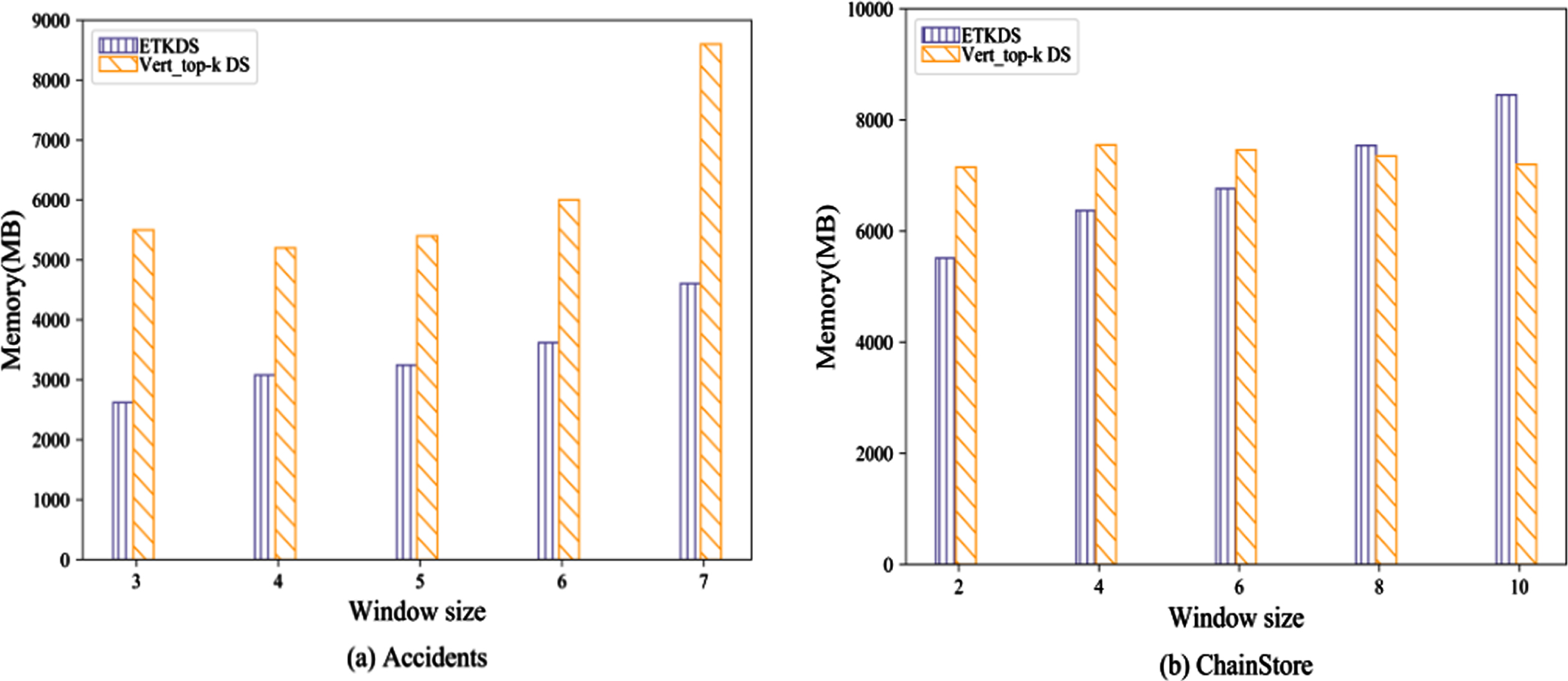
At the same time, ETKDS has the lowest memory consumption on the Accidents dataset according to the memory results shown in Fig. 7, which is significantly lower than the comparison algorithm. When the window is small, it also has lower memory consumption on ChainStore. This is because the pseudo-projection technology adopted by ETKDS does not need to rebuild the projection transaction for each itemset, and when extending an itemset, it only needs to update the original projection to get the sub-projection, but Vert_top-k DS needs to create a new utility-list for each extended itemset. This process requires two utility-lists to join and recreate transaction tuples for the new utility-list, which consumes more memory when the dataset is dense. In addition, Vert_top-k DS generates a large number of intermediate itemsets in different sliding windows because the search space construction mechanism and the pruning strategies used are different between the algorithms. As mentioned earlier, Vert_top-k DS needs to calculate the remaining utility of the intermediate itemset in all the transactions it appears, and creates a corresponding utility-list structure to store this information. Therefore, the Vert_top-k DS storage structure consumes more memory on large datasets such as ChainStore. It is worth noting that the time of ETKDS in the ChainStore dataset and the number of intermediate itemsets are gradually decreasing, but the memory shows an increasing trend as the window size increases. This is because ChainStore is a sparse large dataset with a large number of items. As the window increases, the CIUDataListSW needs to create more batches in the window. At the same time, the batch creation and maintenance costs of each 2-itemset stored in the CUDH _ SW are further increased, which leads to an increase in memory consumption.

Fig. 7

Effect of varying window size on memory.

5.3 Scalability

In this subsection, we select the Accidents and ChainStore datasets in Table 2 to evaluate the scalability of the algorithm ETKDS to verify that the running time and memory consumption of the algorithm do not increase exponentially. The experiment gradually increases the number of mined transactions to test indicators such as time and memory, that is, the number of transactions increases from 50% to 100% of the entire dataset. The comparison algorithm is Vert_top-k DS, and K is fixed at 500.

It can be seen from Fig. 8 that on the dense dataset Accidents, the time advantage of ETKDS over Vert_top-k DS gradually expands as the number of mining transactions increases, and the growth rate of the running time of the Vert_top-k DS is significantly higher than that of the ETKDS. Although the running time of Vert_top-k DS in the later period of the experiment tends to be flat on the sparse dataset ChainStore, and the time growth rate is slightly lower than the ETKDS. However, the average time growth rate of Vert_top-k DS in the entire experiment is still higher than that of the ETKDS. In summary, the ETKDS algorithm proposed in this paper is more time-scalable than Vert_top-k DS, and has greater advantages on dense datasets.

Fig. 8

Scalability test of runtime.

It can be seen from Fig. 9 that the average growth rate of memory usage of ETKDS is lower than that of the comparison algorithm Vert_top-k DS on the dense dataset Accidents, which has better memory scalability. The memory usage of Vert_top-k DS grows more slowly on the dataset ChainStore. This is because although pruning strategies and threshold raising strategies adopted by ETKDS can generate fewer candidate itemsets, the length of a HUI mined is usually very short on the large sparse dataset ChainStore. Besides, there are fewer transactions containing an itemset, which also means that the reduced number of itemsets has limited impact on the memory consumption of utility-list structure and projection structure, so the memory usage of the two algorithms is relatively close on the ChainStore. At the same time, the number of items appearing increases with the increase of mining transactions because the number of items in the dataset ChainStore is far more than that on the dataset Accidents. In addition to the construction of the CIUDataListSW, the CUDH _ SW structure proposed in this paper needs to record information for more itemsets, and the CUCBQ needs to store more candidate minutil. Therefore, the memory scalability of ETKDS on the dataset ChainStore is slightly weaker than that of Vert_top-k DS.

Fig. 9

Scalability test of memory.

6 Conclusions

In this paper, we presented a novel algorithm ETKDS along with a data structure called CIUDataListSW to mine the Top-K high-utility itemsets over a data stream under the sliding window model. ETKDS is based on the Projection-based Pattern-Growth method, using the projected transaction merging technology to reduce the cost of dataset scanning. In the mining process, ETKDS uses the best ordering of items to construct the search space of each sliding window, and designs a reorganization technology for projected transactions in common batches to ensure the correctness and efficiency of the dataset projection process. At the same time, two threshold raising strategies are designed and used based on the CUDH _ SW structure proposed in this paper. Compared with the state-of-the-art algorithm, experimental results on various datasets prove the superior performance of ETKDS. It can also be observed that the threshold raising strategies used in ETKDS can effectively reduce the search space, and the effect is more obvious on dense datasets.

In future work, we will extend this work to be suitable for large-scale distributed computing or parallel computing, and we will also explore how to efficiently mine the closed high-utility itemsets without redundancy over a data stream.

Footnotes

Acknowledgments

This work was supported by the National Nature Science Foundation of China (62062004), the Ningxia Natural Science Foundation Project (2020AAC03216), and the Graduate Innovation Project of North Minzu University (YCX20077).

References

Liu

, Liao

and Choudhary

, A two-phase algorithm for fast discovery of high utility itemsets, the 9th Pacific-Asia Conference on Knowledge Discovery and Data Mining (2015), 689–695.

Tseng

V.S.

, Wu

C.W.

, Shie

B.E.

, et al., UP-Growth: An Efficient Algorithm for High Utility Itemset Mining, the 16th ACM SIGKDD International Conference on Knowledge Discovery and Data Mining (KDD’10) (2010), 253–262.

Tseng

V.S.

, Shie

B.E.

, Wu

C.W.

, et al., Efficient Algorithms for Mining High Utility Itemsets from Transactional Databases, IEEE Transactions on Knowledge and Data Engineering 25(8) (2013), 1772–1786.

Yun

, Ryang

and Ryu

K.H.

, High utility itemset mining with techniques for reducing overestimated utilities and pruning candidates, Expert Systems with Applications 41(8) (2014), 3861–3878.

Liu

and Qu

J.F.

, Mining high utility itemsets without candidate generation, the 21st ACM International Conference on Information and Knowledge Management (2012), 55–64.

Fournier-Viger

, Wu

C.W.

, Zida

, et al., FHM: Faster High-Utility Itemset Mining Using Estimated Utility Co-occurrence Pruning, 21st International Symposium on Methodologies for Intelligent Systems (ISMIS 2014) (2014), 83–92.

Krishnamoorthy

, Pruning strategies for mining high utility itemsets, Expert Systems with Applications 42(5) (2015), 2371–2381.

Yun

, Nam

, Lee

, et al., Efficient approach for incremental high utility pattern mining with indexed list structure, Future Generation Computer Systems 95 (2019), 221–239.

Kim

, Yun

, Baek

, et al., Efficient list based mining of high average utility patterns with maximum average pruning strategies, Information Sciences 543 (2021), 85–105.

10.

Liu

, Wang

and Fung

B.C.M.

, Mining High Utility Patterns in One Phase without Generating Candidates, IEEE Transactions on Knowledge and Data Engineering 28(5) (2016), 1245–1257.

11.

Zida

, Fournier-Viger

, Lin

C.W.

, et al., EFIM: a highly high utility itemsets algorithm for high utility itemset mining, Advances in Artificial Intelligence and Soft Computing (2015), 530–546.

12.

Prasad

J.B.

and Huang

J.W.

, DMHUPS: Discovering Multiple High Utility Patterns Simultaneously, Knowledge and Information Systems 59 (2019), 337–359.

13.

Singh

, Singh

S.S.

, Kumar

, et al., TKEH: an efficient algorithm for mining top-k high utility itemsets, Applied Intelligence 49(3) (2019), 1078–1097.

14.

Sohrabi

M.K.

, An efficient projection-based method for high utility itemset mining using a novel pruning approach on the utility matrix, Knowledge and Information Systems 62(11) (2020), 4141–4167.

15.

Zihayat

and An

, Mining top-k high utility patterns over data streams, Information Sciences 285(1) (2014), 138–161.

16.

Dawar

, Sharma

and Goyal

, Mining Top-K high-utility itemsets from a data stream under sliding window model, Applied Intelligence 47(12) (2017), 1240–1255.

17.

Ryang

and Yun

, High utility pattern mining over data streams with sliding window technique, Expert Systems with Applications 57 (2016), 214–231.

18.

Jaysawal

B.P.

and Huang

J.W.

, SOHUPDS: a single-pass one-phase algorithm for mining high utility patterns over a data stream, the 35th ACM/SIGAPP Symposium on Applied Computing (SAC ’20) (2020), 490–497.

19.

Tang

, Liu

and Wang

, A New Algorithm of Mining High Utility Sequential Pattern in Streaming Data, International Journal of Computational Intelligence Systems 12(1) (2018), 342–350.

20.

Hackman

, Huang

, Yu

P.S.

, et al., Mining Emerging High Utility Itemsets over Streaming Database, the 16th International Conference on Advanced Data Mining and Applications (2019), 3–16.

21.

Duong

Q.H.

, Liao

, Fournier-Viger

, et al., An efficient algorithm for mining the top-k high utility itemsets using novel threshold raising and pruning strategies, Knowledge-Based Systems 104 (2016), 106–122.

22.

Krishnamoorthy

, Mining top-k high utility itemsets with effective threshold raising strategies, Expert Systems with Applications 117 (2019), 148–165.