Detection and diagnosis of age-related macular degeneration using recurrent neural network with cloud architecture and internet of things

Abstract

Age-Related Macular Degeneration is a progressive, irreversible eye condition that causes vision loss and impairs quality of life. The lost potential of the optic nerve cannot be regained, but a patient with Age-Related Macular Degeneration must have early diagnosis and treatment in order to prevent visual loss. The diagnosis of Age-Related Macular Degeneration is based on visual field loss tests, a patient’s medical history, intraocular pressure, and a physical fundus evaluation. Age-Related Macular Degeneration must be diagnosed early in order to avoid irreparable structural damage and vision loss. The objective of the proposed study is to develop a new optimization-driven strategy-based recurrent neural network using the Internet of Things for the identification of age-related macular degeneration. The Recurrent Neural Network (RNN) classifier is trained using the Particle Swarm Optimization (PSO) technique included into the RNN-IoMT. Initially, the input picture is sent through pre-processing in order to remove noise and artefacts. The generated preprocessed picture is simultaneously sent to optical disc detection and blood vessel detection. In addition, picture level characteristics are extracted from the image that has been preprocessed. Finally, the image-level, optic disc-level, and blood vessel-level features are retrieved and compiled into a feature vector. The acquired feature vector is fed into the RNN classifier, with the suggested PSO used to train the RNN for Age-Related Macular Degeneration detection via the Internet of Medical Things. The suggested PSO+RNN exhibits better performance with enhanced precision of 97.194%, sensitivity of 97.184%, and specificity of 97.2044%, respectively.

Keywords

Wearables internet of things teleophthalmology deep learning fundus images

1 Introduction

The retina coats the inside of the eyeball’s rear surface. It takes the picture that the lens forms, processes it into electrical impulses, and transmits them to the brain so that it may be recognized visually [1]. Photoreceptors, or light-sensitive cells, are found in the retina and provide visual information to the brain through the optic nerve. Located in the retina’s center, the macula is an oval region (approximately 5–6 mm in diameter) that controls spatial resolution and color vision. It’s crucial to one’s eyesight since that’s where the lens focuses light. Humans have their best vision in a dip or pit inside the macula called the fovea. Diseases of the macula include AMD and DME, two major forms of retinal degeneration caused by diabetes. In particular, age-related macular degeneration (AMD) is a neurological condition that causes central vision impairment or loss. It is unclear what causes AMD, although there are known, unavoidable risk factors, such as age (more prevalent in the elderly), sex (more common in women), family history, and race (more commonly seen among Caucasians than other races). It affects one in twenty people and is the fourth most common eye condition leading to blindness worldwide. AMD affects 8.7 percent of the global population; the number of patients with the condition is predicted to rise from the current estimate of 196 million in 2020 to 288 million by 2040 [2].

Since there are currently no effective therapies for AMD, many people are turning to novel methods to slow the disease’s development. As AMD worsens, it may affect normal visual functions including recognizing shapes, driving, reading, and writing. Researchers all around the globe are hard at work trying to perfect more effective methods of identifying ocular disorders like AMD so that patients may maintain their eyesight and quality of life for as long as possible. Fundoscopy, fluorescein angiography, Optical Coherence Tomography (OCT), and tonometry are the most prominent non-invasive imaging procedures used to detect/screen for AMD. Several recent studies have examined the effectiveness of OCT images in identifying a variety of eye illnesses [3]. Information useful for diagnosing AMD is included in the layers’ varied thicknesses and abnormalities. Normal, dry, and moist AMD may all be distinguished from one another in color OCT scans.

Time-Domain Optical Coherence Tomography (TD-OCT) [4] and Spectral-Domain OCT are the two basic OCT subtypes (SD-OCT). Numerous investigations, like the one described here, have shown that SD-picture OCT’s resolution is superior to that of TD- OCT’s. Despite OCT’s promising potential for enhanced screening of AMD and related biomarkers, the sheer amount of data generated renders manual analysis prohibitive. Manual evaluation of OCT data may be time-consuming and prone to mistakes in detection, which is problematic given the high volume of patients seen by an ophthalmologist. By providing quantitative and objective metrics that might help in clinical choices, automated/computer-aided diagnostic models can relieve some of the burden placed on ophthalmologists. Experts may save time by focusing on the suspicious areas identified by the automation tool, rather than sifting through the whole OCT picture, and statistical and Machine Learning (ML) [5] models are increasingly seen as beneficial for facilitating the first screening of the OCT images. Pattern recognition and in-depth analysis of OCT images at scales and rates much beyond what is conceivable by hand are both within the reach of such models. OCT images are processed using statistical and ML algorithms in this suggested study for the purpose of binary categorization of AMD (AMD detection). The AMD levelling (beginner, intermediate, or advanced) may be saved for later.

The primary goal of this research was to improve statistical and ML techniques for detecting AMD in OCT images. In this process, we were able to complete the following:

A statistical technique was presented for the diagnosis of dry AMD. Drusen identification relied on a height measurement produced by subtracting the RPE from the baseline (the individual patient’s natural eye curvature). Various statistical methods were used to estimate RPE and baselines.

It was suggested using a multiscale convolutional neural network (CNN) with seven convolutional layers to sort retinal images into AMD (dry and wet) and normal kinds. The multiscale convolution layer allowed for the generation of many different local structures throughout a range of 5 kernel sizes. The sigmoid function was chosen as the classifier for this suggested network.

Convolutional layers were utilized in an AMD detector that was a multipath CNN. The sigmoid function was utilized as a classifier, and the multipath convolution layer made it possible for global structures with a large filter kernel.

Images were classified as having AMD or being normal using a mix of dual-path and poly-scale structures. Large and small filter kernels were used to extract the global and local characteristics, respectively. For this purpose, we next turned to the sigmoid activation function.

Feature extraction was carried out using a framework that included both multipath and multiscale structures. For classification, ten-fold cross-validation was used using three different classifiers (SVM, MLP, and RF).

The organization of paper is as follows; Section 2 includes related work; section 3 includes methodology of proposed work; section 4 includes experimental results and analysis; section 5 includes conclusion and future work.

2 Related work

Discrete wavelet analysis characteristics of the OD were derived by [6]. Bit plane analysis is used to pinpoint the OD. The key characteristics were calculated using Principal Component Analysis (PCA) and evolutionary attributes. The variation mode decomposition approach was used by [7] to extract characteristics including Kapoor, Reyni, Yager, and fractal dimension. The Relief technique is used to pick out prominent characteristics. [8] It used a retinal fundus picture and used a random transform to isolate HOS Cumulant characteristics. Linear Discriminant Analysis (LDA) was used for feature reduction in order to sort the images into those with Age-Related Macular Degeneration and those without. Features such as the variance, mean, skewness, energy, kurtosis, Shannon were derived from Gabor transform coefficients by [9]. Gabor transform coefficients aided in detecting even the most minor of alterations to the picture. The entropy, Bhattacharya algorithm, t-test, and Wilcoxon test were only some of the statistical tools used to determine grades for these characteristics. Using vascular convergence and feature based weighted maps, [10] suggested a regional based image feature model that localizes the OD. These features include gradient, Gaussian, Gabor, and wavelet. In order to evaluate and choose characteristics, [11] used wavelet-based energy features. To classify AMD, [12] used a convolutional neural network (CNN) with 18 layers. In order to estimate the class of the fundus picture, a hierarchical mapping of the pixels from the input image is used. The hospital dataset contains 1426 images, which are used to train the CNN model from scratch. For a big set of photos, the model performs optimally.

Using Gradient Information Scales and Orientations (GIST) and a pyramid histogram of oriented gradient. features [13] created a method to identify Age-Related Macular Degeneration. The GIST gives the picture a representation based on its geometric characteristics. The pyramid represents the spatial details, while the histogram of gradient captures the overall contour of the picture. From the total of 1448 characteristics, PCA is used to extract the most salient ones. First, [14] used a Laplacian of Gaussian filter to pinpoint OD in the red channel. The filter uses the pixels with a 60% response rate to determine the potential OD area. Each potential area has a window centered on it to determine the density of blood vessels there. The OD region is defined as the area with the greatest concentration of blood vessels.

A multivariate with m-medoids and fisher discriminate analysis in feature enhancement are employed for classification. Pre-processing the fundus images using histogram equalization and random transform, [15] created a technique for detecting Age-Related Macular Degeneration. Higher-order spectral and discrete wavelet transform characteristics are retrieved from the preprocessed fundus picture. A risk index for Age-Related Macular Degeneration is constructed on the basis of the relevance of the retrieved characteristics. To accomplish this goal, [16] used principal component analysis (PCA) on intensity values for pixels. They used things like the image’s texture and B-Spline coefficients from the Fast Fourier Transform (FFT) to use as features. These characteristics were used to calculate the Geographic Risk Index (GRI) for age-related macular degeneration.

In order to diagnose Age-Related Macular Degeneration, [17] integrated textural data with Higher Order Spectra (HOS) features from the fundus image. Using Discrete Wavelet Transform (DWT) and HOS characteristics extracted from fundus images, [18] distinguished between normal and Age-Related Macular Degeneration images. Intensity, cumulative zero count local binary pattern, directional differential energy, and Shannon entropy are only few of the properties that [19] measured. The color photos were converted to their grey scale counterparts using adaptive histogram equalization by [20, 21]. The greyscale images are processed via a filter bank which stand in for the fundamental components of natural images. Higher order spectra are used to extract spectral information from the textons, which are then used to distinguish between photos of people with and without Age-Related Macular Degeneration. Extraction of geometric (clinical) and textural data may provide more accurate findings than utilizing solely CDR for identifying Age-Related Macular Degeneration. There is a dearth of state-of-the-art methods that use CDR and ISNT rule-based clinical knowledge of AMD in addition to characteristics derived based on intensity or color for differentiating fundus images.

3 Proposed methodology

Many different automated methods have been developed for detecting optic discs by analyzing parameters such as the disc’s size, contrast, shape, and grayscale. When presented with high-quality photos in which the optic disc is clearly visible and exhibits predicted traits, the traditional approaches excel at its discovery. Retinal diseases cause aberrant alterations in the images, which ultimately leads to failure. Multiple strategies have been used for quite some time to identify illnesses and segment retinal components including the optic disc and blood vessels. However, automated optic disc and blood vessels segmentation suffers from performance degradation since images are acquired under widely changing circumstances of resolution, lighting, field of view (FOV), and overlap tissue from the retina. Previous methods relied on a combination of filters and thresholding algorithms to locate the points where blood veins met the retina. Because of the fundus image’s noise and distortions, traditional edge detection masks, such as the Kirsch template, failed to accurately recognize blood vessels. Therefore, it is necessary to provide a practical system for detecting blood vessels and the optic disc that can maintain the variety of artery and disc forms. Figure 1 presents a high-level block diagram of the PSO-RNN method.

Fig. 1

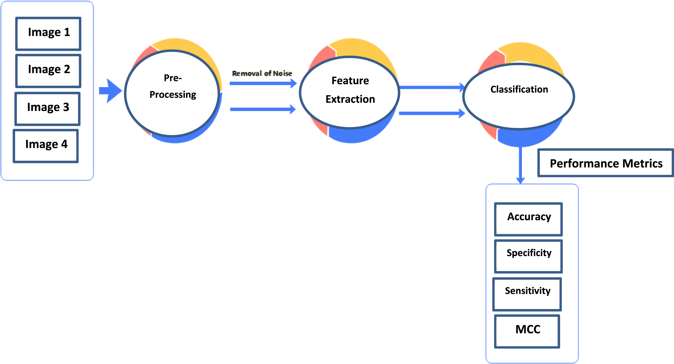
Block diagram of PSO-RNN IoMT technique.

3.1 Image acquisition

Wearable OphthoAI-IoMT headsets with integrated cameras and AMD-ResNet deep CNN applications can assess AMD disease severity. Both built-in AI and a cloud-based Artificial Intelligence and Data Analytics Service are available for use in the headset’s analysis and conclusion-drawing processes. Users’ data is encrypted, deleted, or retained locally in a safe manner once they have given their consent. A cloud computing (CC) framework that controls and connects several OphthoAI-IoMT headsets, secure fundus image broadcast, secure forbearing virtual warehouse, monitoring and metering of compute capacity, etc.

3.2 Image preprocessing

Pre-processing is crucial because it ensures that incoming retinal images can be processed without any hiccups. In order to make a picture suitable for detection, pre-processing is used. In addition, the pre-processing phase is used to get rid of any noise in the original picture. Additionally, pre-processing is seen as image augmentation since it may enhance an image’s contrast for efficient ARMD detection. Optic disc detection and blood vessel detection components are applied simultaneously to the preprocessed images to mine the relevant features for ARMD detection.

Assume there is a collection of h ⩾ 3 points in 2-space labelled as (u₁, v₁) (u₂, v₂) , …, (u_k, v_h). The motive is to determine a circle that best represents the data. Using the circle defined by (u - d) ² + (v - f) ² = r², there is a requirement to detect values for center (d, f) and radius r to best describe the circle fitting.

Thus, the circle fitting using (u - d) ² + (v - f) ² = r² to the points (u₁, v₁) (u₂, v₂) , …, (u_k, v_h) is obtained by adding the squares of distance from the points to the circle and is represented as, $SS (d, f, r) = \sum_{e = 1}^{h} {(r - \sqrt{{(u_{e} - d)}^{2} + {(v_{e} - d)}^{2}})}^{2}$ (1) When data is transformed into an exponential form, the exponential kernel may be identified using the formula (2). $l_{1} = \exp [\frac{h^{2}}{2 K_{d}^{2}}]$ (2) The kernel is obtained by normalizing the vector, l-1, and this is represented by the Equation (3), $f_{1} = \frac{[\frac{1}{p} \sum_{k = 1}^{p} \max (l_{1}) - l_{1}] - l_{1}}{\sum_{k = 1}^{p} \max (l_{1}) - l_{1}}$ (3) The input, already-processed picture is rotated by a total of p degrees to generate p identically-sized copies. Finally, a sparking picture is created, and it may be written as Equation (4), $α_{men} (k, m) = \frac{α_{l} + α_{min} (k, m)}{α_{max} (k, m)} 255$ (4) Where, α_min (k, m) = min [s₁ (k, m) , s₂ (k, m) , …, s_p (k, m)], and

$\begin{matrix} α_{max} (k, m) \\ = max [s_{1} (k, m), s_{2} (k, m), \dots, s_{p} (k, m)] \end{matrix}$ (5)

To get the optimal threshold, a sparking picture is employed. This procedure generates a matrix known as a “neighbor pixel,” where the rows represent the values of the current pixel and the columns represent the values of its neighbours. The fun function is used to compute each pixel’s value between 0 and 255 in order to find the optimal threshold. Expressions for matrices E and F in terms of the cutoff B may be found if, $\begin{matrix} E \Leftarrow [B \times B] \\ F \Leftarrow [(255 - B) \times (255 - B)] \end{matrix}$ (6) Renya entropy is used to assess the information gain between E and F given a threshold value of B. Renya’s expression for the entropy of, E_k, $R_{e} (E) = \frac{1}{1 - α} log (\sum_{k = 1}^{p} P (E_{k})')$ (7) Where, j signifies real number, p stands for total number of images; 1 ⩽ k ⩽ p, P (E_k) indicate probability of E_k. The Renya entropy of F_k is expressed as, $R_{ɛ} (F) = \frac{1}{1 - α} log (\sum_{k = 1}^{F} P (F_{k})')$ (8)

Where, j represent real number, p symbolize total images; 1 ⩽ k ⩽ p, P (F_k) indicate the probability of F_k, and the Renyi entropies of E and F are symbolized as R_e (E) and R_e (F).

The ideal threshold value may be selected by adding up the entropies. $G = R_{e} (E) + R_{e} (F)$ (9)

The segments needed to locate the optic disc in the input retinal picture are produced after the Renya-based sparking approach has been used.

3.3 Feature extraction

i) Mean: The equation for this measurement, which estimates the typical number of pixels in a picture, is, $α = \frac{1}{∣ p (R_{w} ∣} \times \sum_{n = 1}^{| ρ | R_{n} ∣} p (R_{n})$ (10)

In this case, m represents the total number of segments, R_n represents the pixel value of each segment, and n represents the total number of pixels in that segment as ∣p (R_w).

ii) Variance: Calculating the variance from the mean yields the following formula: $σ = \frac{\sum_{n = 1}^{1} | R_{n} |}{p (R_{n})}$ (11)

iii) Standard deviation: The sign stands for the square root of the variance.

iv) Kurtosis and the skewness: Kurtosis quantifies how sharp a peak is on average. Skewness and kurtosis, when used together, provide a numerical description of the shape of the thing. The skewness quantifies how off-center the distribution of probabilities is, whereas the kurtosis assesses how heavily weighted any one peak is in the distribution.

v) Entropy: The entropy is maximized, and the degree of uncertainty in the data is measured. Favoring the correctness of the action drives the entropy. Entropy is used to isolate the differences between adjacent or related pixels. The entropy was also used to describe the degree of adaptation at each individual pixel. Comparison of image details may be improved by analyzing the entropy of each pixel.

3.4 Image classification

Recurrent neural networks (RNNs) include just a single recurrent loop known as a feedback loop. The feedback loops stand for recurrent cycles in time. A training dataset consisting of input-target pairs is required for the RNN to work. Through the use of a weight optimization strategy, RNN is able to close the gap between its output and its target audience. An RNN is able to process consecutive inputs because its recurrent hidden state uses the previous layer’s output as the activation function.

Therefore, the network displays temporal aspects of change. Furthermore, the recurrent layer permits feeding the information from earlier time steps and integrating the resulting output with the input vector sequence from the current time step with, v-rit. time, such that,...,,H-V1.,,J-F.,,J-V+1.,....where, the term, H-r. refers to selected features obtained from the developed model. In the RNN’s hidden layer, the input is connected to hidden units by links described by the weight matrix, w-,a. Since, there are X hidden units making up the hidden layer, A₁ = β (u₁) State space, or the memory of the system, is defined by the hidden layer, which is provided by, $A_{1} = β (u_{1})$ (12)

The equation of system memory v_v in the state space is expressed by, $v_{v} = σ_{Sa} J_{u} + σ_{Ba} H_{v - 1} + γ_{g}$ (13)

Where, the system memory is denoted as ν_v, the activation function is indicated as β, the term λ_g represents the bias vector of the hidden units, ϖ_M refer to weight relating input and the hidden layers, the term ϖ_Aa signifies the weight with two hidden layers. Hence, output vector expressed as, $P_{v} = β^{'} (σ_{un} g_{v - 1} + γ_{f})$ (14)

Where, the term γ refers to the bias of the output layer, and β denotes activation function. Figure 2 depicts the DBN method’s construction.

Fig. 2

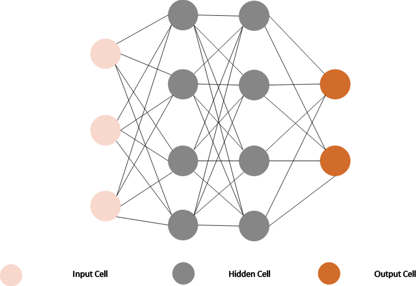
RNN structure.

a) Initialization: The population of chicken is initialized in first step with their related parameters. $D = {D_{1}, D_{2}, \dots, D_{e}, \dots D_{n}}$ (15)

Where, the term D_c signifies the c^1k chicken location, and the total population is denoted as h. b) Error computation: The optimal solution is identified based on fitness function, which is known to be optimization problem, and hence, the solution with minimal Mean Square Error (MSE) is chosen as optimal solution, and equation is given below. $M S^{wr} = \frac{1}{b} \sum_{e = 1}^{b} {[Q, - Q_{e}^{*}]}^{2}$ (16)

Where, the expected and the predicted output is denoted as Q, and $Q_{α}^{*}$ , the total data samples are indicated as e.

c) Update Equation Determination: Better convergence rates and overall performance are achieved by using the CSO method. Since the CSO’s algorithmic structure is straightforward, it requires fewer parameters for fine-tuning when the solution is calculated. The CSO algorithm’s typical update equation is, $D_{e, ɛ} (e + 1) = D_{e, ɛ} (e) * (1 + Randn (0, χ^{2}))$ (17)

3.5 Hyper-parameter optimization

Linear, Gaussian, quadratic, and cubic kernel’s functions are shown in Table 1. The kernel function of the Support Vector Machine (SVM) classifier using a Gaussian distribution is a weighted linear combination. In the input feature space, the Gaussian kernel computed using support vector machines is a function that decays exponentially over time. This causes the kernel function to have hyper-spherical outlines, with its maximum value located at the support vector and decaying equally in all directions around the support vector.

Table 1
Common kernel functions with functional expressions

Kernel function name Formula

Gaussian K (x_i, x_j) = exp(- ∥ x_i - x_j) ∥ ²)

Linear K (x_i, x_j) = x_i^′x_j

Quadratic K (x_i, x_j) = (x_i, x_j + 1) ²

Cubic K (x_i, x_j) = (x_i^′x_j + 1) ³

Kernel function name	Formula
Gaussian	K (x_i, x_j) = exp(- ∥ x_i - x_j) ∥ ²)
Linear	K (x_i, x_j) = x_i^′x_j
Quadratic	K (x_i, x_j) = (x_i, x_j + 1) ²
Cubic	K (x_i, x_j) = (x_i^′x_j + 1) ³

After putting the classifier through its paces, it was discovered that the Gaussian kernel function yielded the best results when attempting to categories retinal illnesses. PCA-SVM aims to do the following things.

The goal is to narrow down the vast feature space to just the most important aspects and discard the rest.

To unearth novel informative characteristics and highlight the robust patterns with the greatest variation.

Reduce the computational complexity of support vector machines (SVMs) by feature extraction and dimensionality reduction. More than two classes may be classified with the help of multi-class SVM. In order to categories data points into distinct sets, hyperplanes are constructed. The original multiclass issue is broken down into many binary ones. We may write down the hyperplane as, $f_{h} (x) = (w_{c} \cdot x_{1}) + b_{c}$ (18)

The weighted vector, w-c. is the product of the bias, b-c, and the support vector (x-i). The suggested approach designates normal vision as a feature vector size of 0, age-related macular degeneration as 1, and dry eye as 2. Extracted characteristics include CDR, BVR, NRR, DDLS, and exudates area from a variety of datasets. All of the relevant datasets have had the suggested strategy for characterizing them tested through trial and error. Seven of the forty photos in the DRIVE dataset. Overfitting towards DR class might result from this. There are 45 photos total, with a balance between normal, DR, and ARMD in the HRF collection. There are a total of 101 photos in the DRISHTI-GS collection, and 70 of them have ARMD. Similarly, there are a total of 81 images and 51 DR in the STARE dataset. Overfitting towards a class may be avoided by training a small dataset using an SVM classifier using 10 rounds of cross-validation.

4 Performance validation

In the realm of eye illness diagnosis, ground-truth photographs created and approved by an ophthalmologist are often used to verify the accuracy of the segmentation. The effectiveness of the suggested segmentation algorithm is measured by contrasting the algorithm’s results with those of human experts. The research is checked against five distinct datasets (STARE, DRIVE, HRF, DRISHTI-GS, and PSGIMSR). Comparing the MFCM output to that of three other segmentation methods— K-means clustering maximal entropy thresholding (MET) and fuzzy c-means (FCM) clustering is used to verify the segmentation algorithm’s efficacy.

Fig. 3

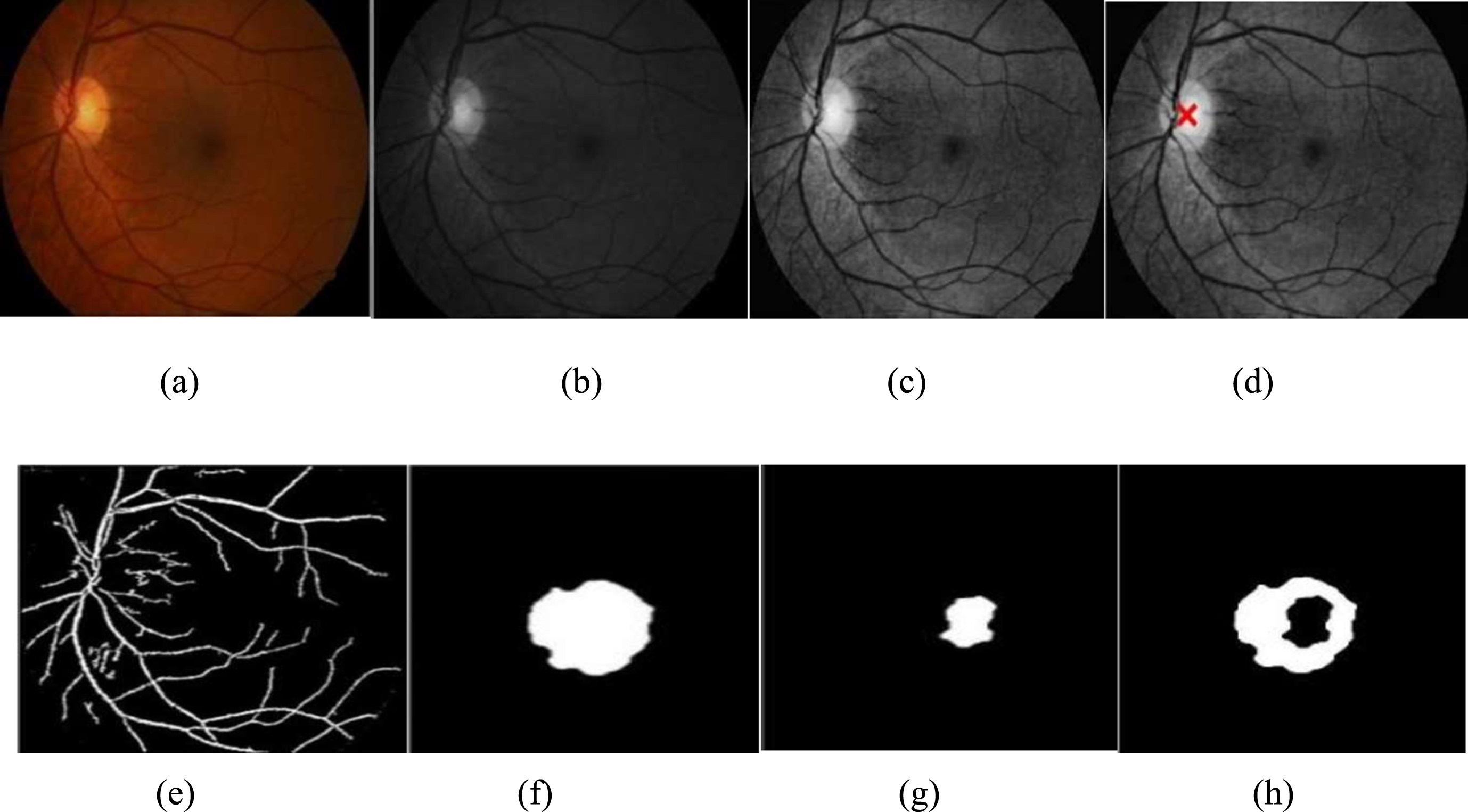
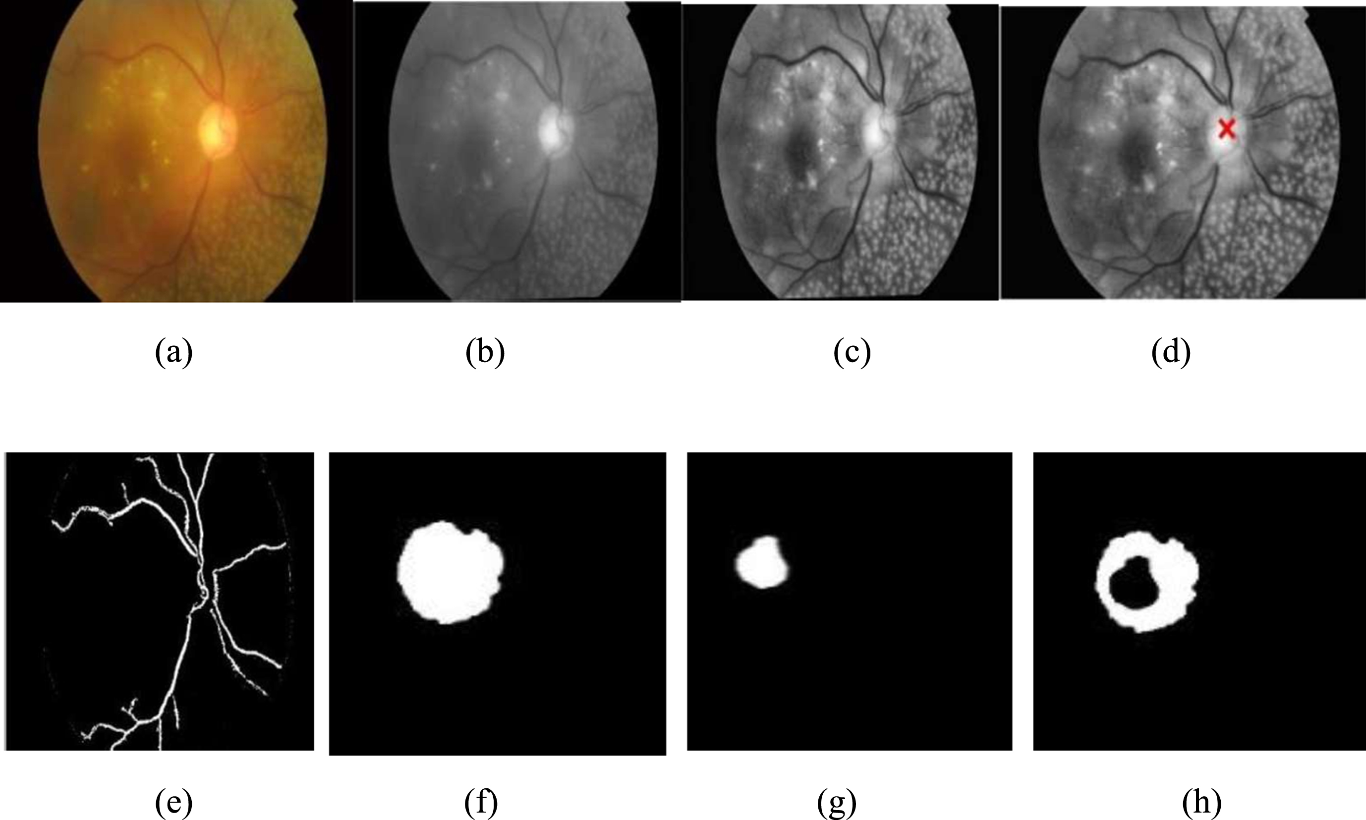
(a) Input image of a normal eye, (b) Noise removal, (c) Contrast Limited Adaptive Histogram Equalization, (d) Localization of OD, (e) Blood vessel segmentation, (f) Segmentation of OD, (g) Segmentation of OC, (h) Neuro Retinal Rim.

Case study images and analysis findings for the suggested system for a variety of fundus images are shown in Fig. 4(a)-(b). The input fundus picture is shown in Fig. 4(a). The segmentation process begins with the improved input picture shown in (b) and (c) of Fig. 5. Because to the pre-processing, distinguishing between OC and OD borders is very evident. Blood vessel segmentation (Fig. 5(e)) and OD localization (Fig. 5(d)) are shown below. The MFCM algorithm’s work in segmenting the OD and OC is seen in Fig. 5(f) and (g). The neuroretina rim is seen in Fig. 5(h). The segmentation strategy for photos from a different dataset is shown in Figs. 4 and 5.

Fig. 4

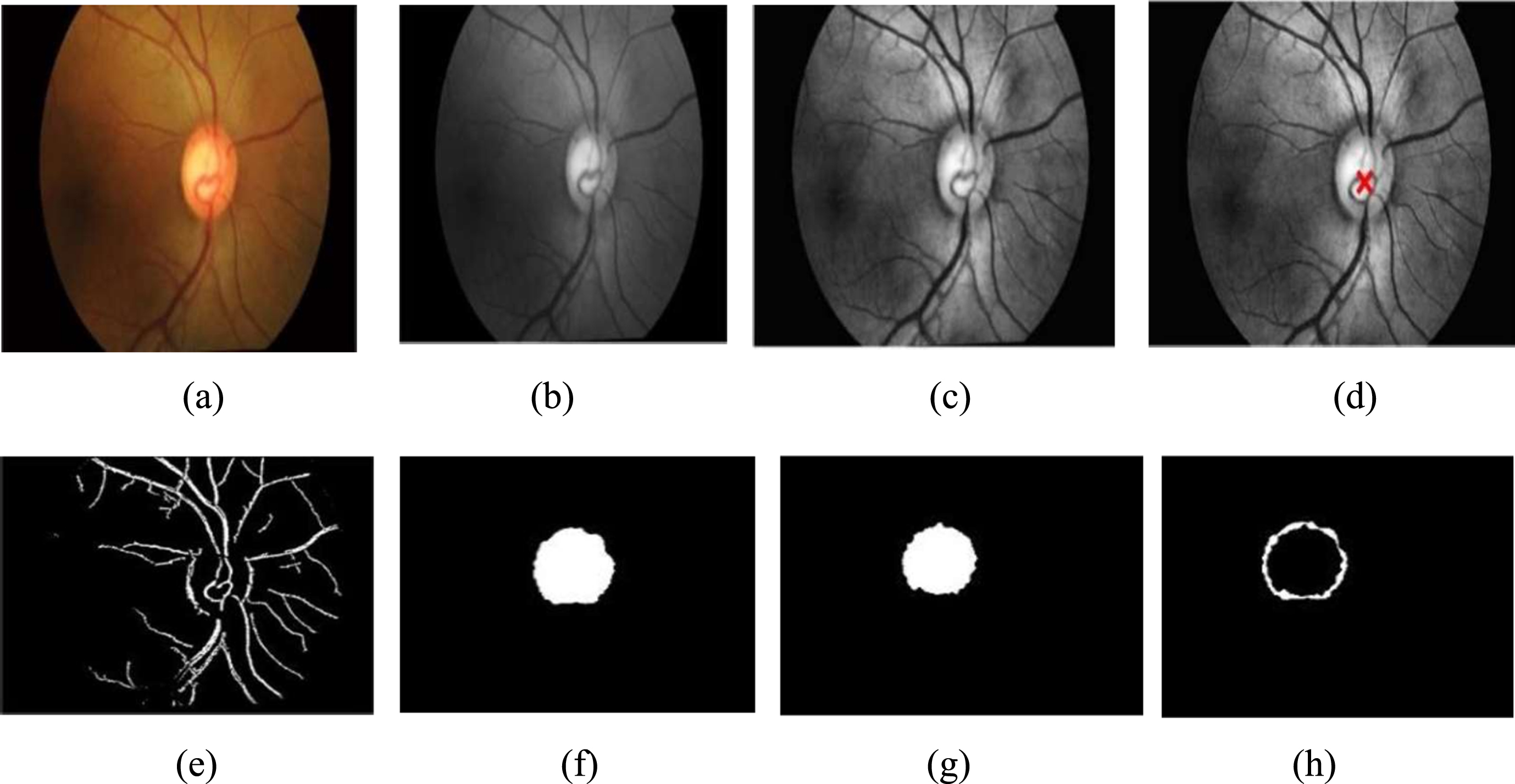
(a) Input image affected by ARMD, (b) Noise removal, (c) Contrast Limited Adaptive Histogram Equalization, (d) Localization of OD, (e) Blood vessel segmentation, (f) Segmentation of OD, (g) Segmentation of OC, (h) Neuro Retinal Rim.

Fig. 5

(a) Input image affected by DR, (b) Green channel extraction, (c) Contrast Limited Adaptive Histogram Equalization, (d) Localization of OD, (e) Blood vessel segmentation, (f) Segmentation of OD, (g) Segmentation of OC, (h) Neuro Retinal Rim.

The mask used for neuroretina rim and blood vessel extractions in each quadrant is shown in Fig. 4. In the retinal picture, the nasal and temporal areas are located in the upper left and lower right quadrants, respectively. The neuroretina periphery is shown in Fig. 4(a). The neuroretina region in the upper eye is shown in Fig. 5(b). Multiplying the mask picture by the size of the neuroretina rim yields this result. Figure 3.11 shows the outcomes of a similar method applied to the remaining two quadrants (c)-(e).

Fig. 6

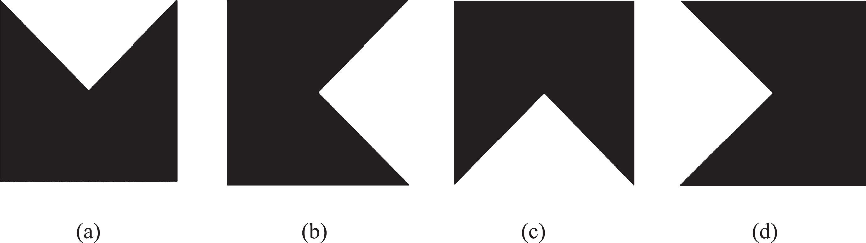
(a) Mask for superior, (b) Mask for temporal, (c) Mask for inferior, Mask for nasal.

Fig. 7

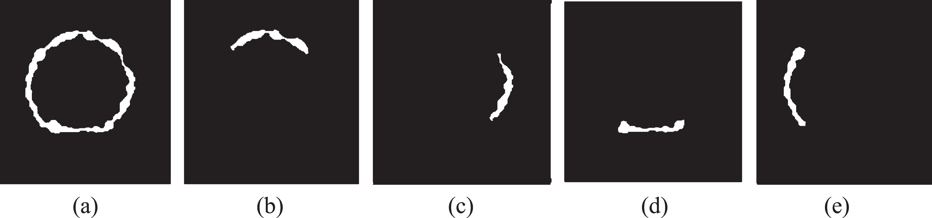
(a) Segmented Neuro Retinal Rim (NRR) area, (b) NRR area in superior, (c) NRR area in temporal, (d) NRR area in inferior, (e).

Fig. 8

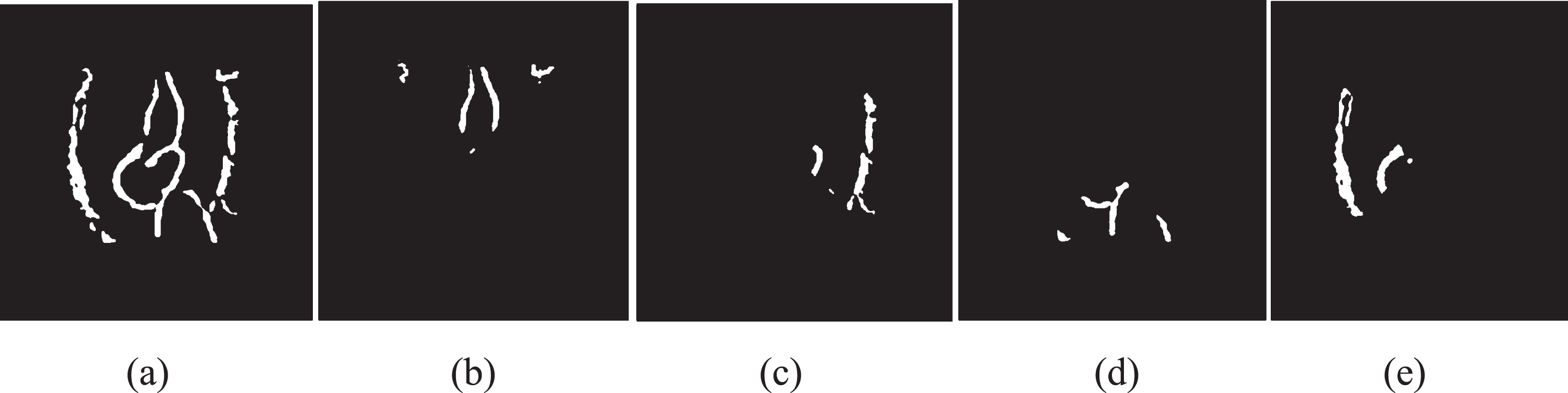
(a) Extracted Blood Vessel Ratio (BVR), (b) BV in superior, (c) BV in temporal, (d) BV in inferior, (e) BV in nasal.

Fig. 9

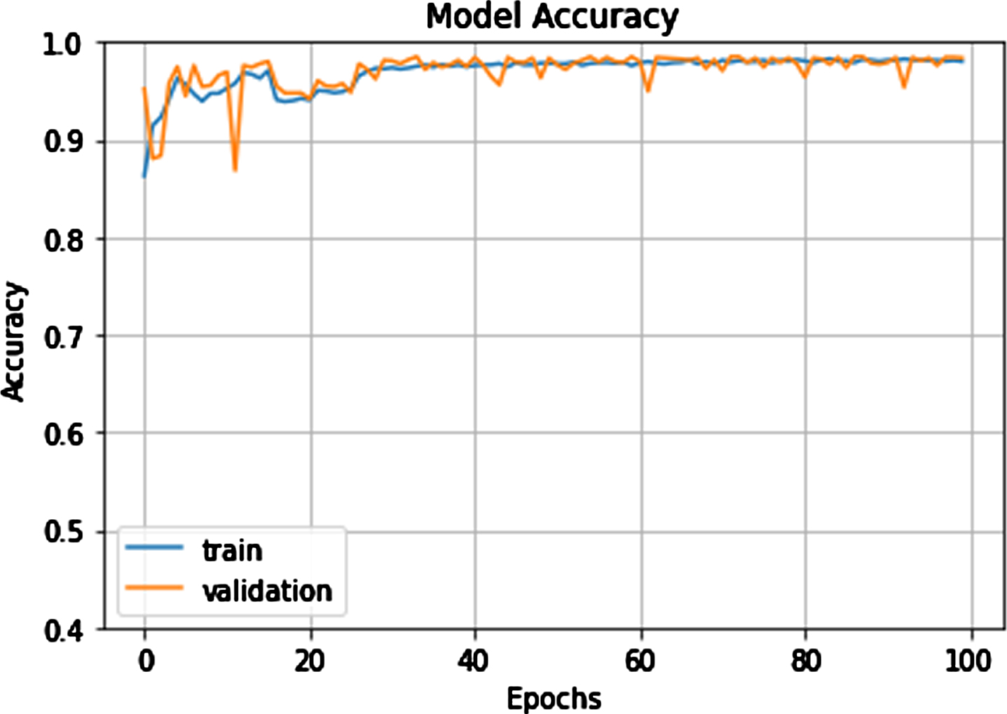
Model training Accuracy and testing Accuracy.

In this part, we analyses how changing the picture size from 512 to 2048 affects the performance of a PSO-based RNN on dataset-2. Accuracy study of PSO-based RNN is shown in Fig. 5.12. Accuracy is 72.62 percent for the PSO-based RNN with hidden layer 5, 76.05 percent for the PSO-based RNN with hidden layer 10, 82.61 percent for the PSO-based RNN with hidden layer 15, 86.44 percent for the PSO-based RNN with hidden layer 20, and 89.68 percent for the PSO-based RNN with hidden layer 25 on 50% training data. For 60% training data, the accuracy of the PSO-based RNN with hidden layer 5 is 75.01 percent, the PSO-based RNN with hidden layer 10 is 85.63 percent, the PSO-based RNN with hidden layer 15 is 89.05 percent, and the PSO-based RNN with hidden layer 25 is 92.52 percent.

Accuracy for 70 percent training data is 76.86 percent for the PSO-based RNN with hidden layer 5, 83.28 percent for the PSO-based RNN with hidden layer 10, 86.25 percent for the PSO-based RNN with hidden layer 15, 89.24 percent for the PSO-based RNN with hidden layer 20, and 92.72 percent for the PSO-based RNN with hidden layer 25. The PSO-based RNN with hidden layer 5 achieves an accuracy of 0.88%, the PSO-based RNN with hidden layer 10 achieves an accuracy of 0.86%, the PSO-based RNN with hidden layer 15 achieves an accuracy of 0.88%, the PSO-based RNN with hidden layer 20 achieves an accuracy of 0.90.31%, and the PSO-based RNN with hidden layer 25 achieves an accuracy of. 92.31%.

PSO-based RNN specificity study on dataset-2 with 512x512 images is shown in Fig. 11.

Fig. 10

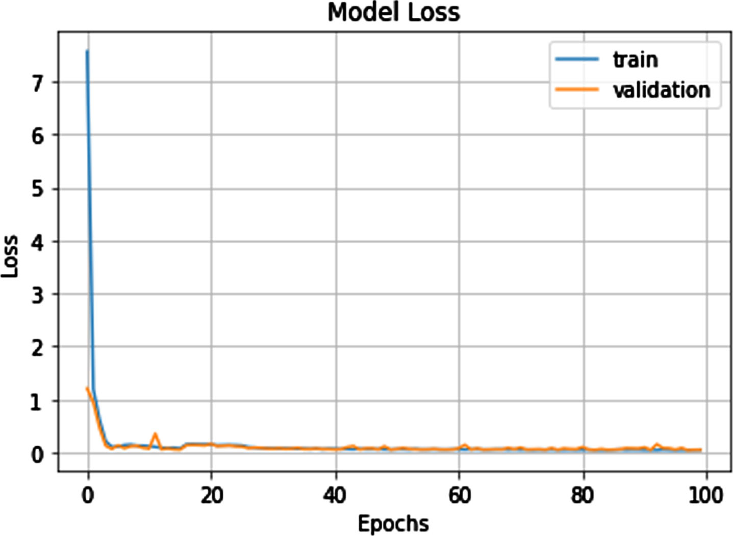
Training and Testing of Model Loss technique.

Fig. 11

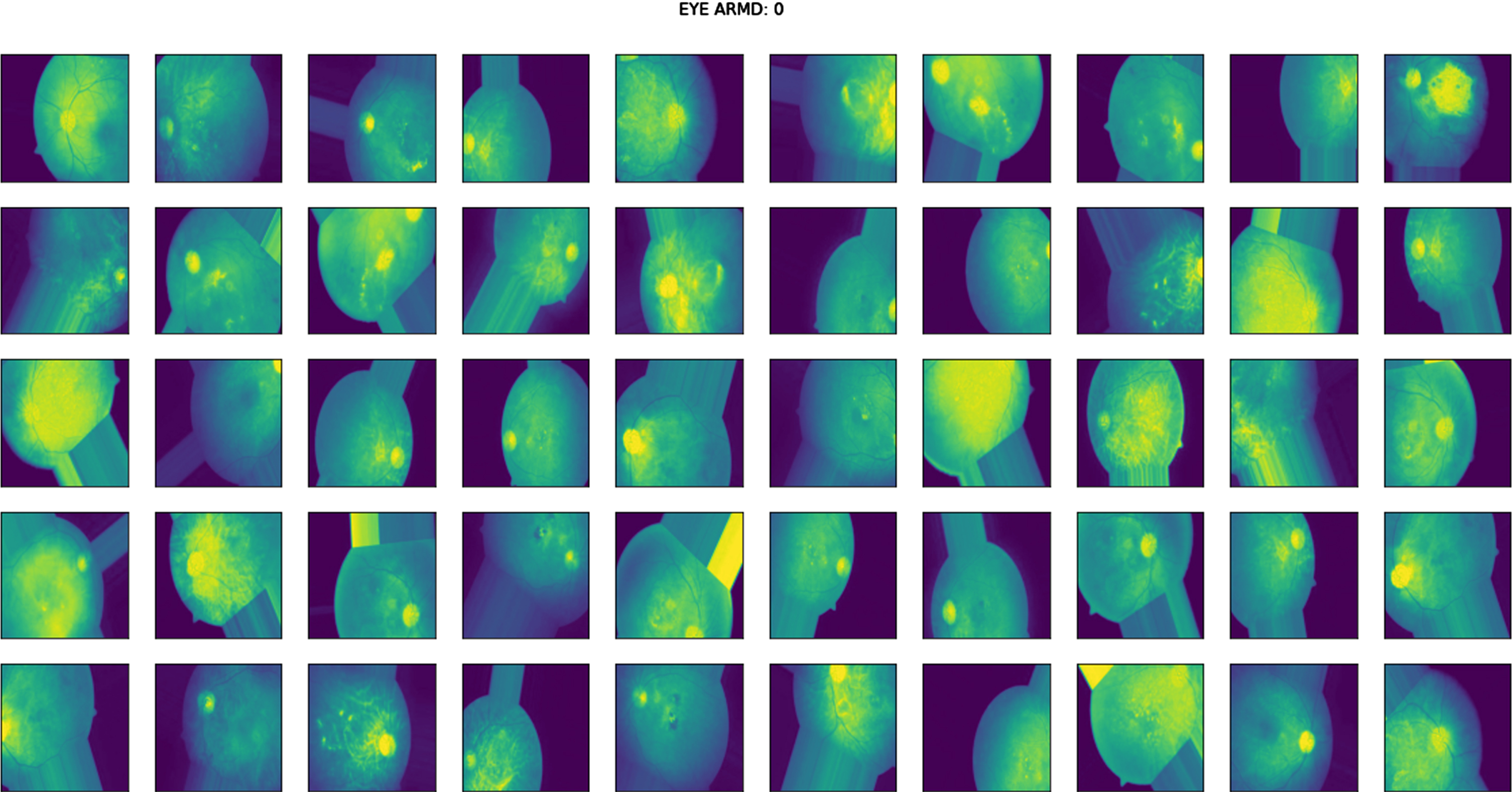
Image Classification using PSO-RNN.

Specificity is 70.67 percent for PSO-based RNNs with hidden layer 5, 76.03 percent for PSO-based RNNs with hidden layer 10, 84.43 percent for PSO-based RNNs with hidden layer 15, 88.56 percent for MFV-DBNs with hidden layer 20, and 91.18 percent for MFV-DBNs with hidden layer 25 on 50 percent training data. Specificity is 75.31% for 60 percent training data using a PSO based RNN with hidden layer 5, 80.74% using a PSO based RNN with hidden layer 10, 87.34% using a PSO based RNN with hidden layer 15, 90.34% using a PSO based RNN with hidden layer 20, and 92.98% using a PSO based RNN with hidden layer 25.

Fig. 12

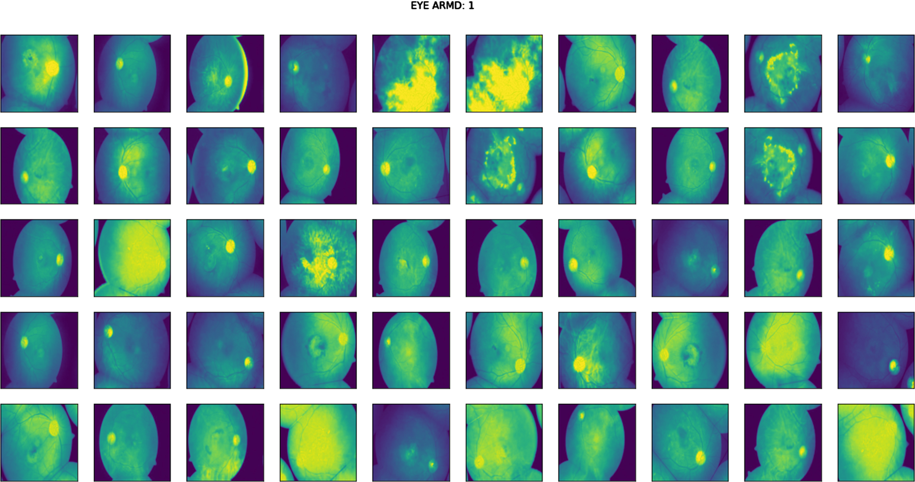
Image Classification using PSO-RNN with ARMD dataset.

Specificity is 78.23% for 70 percent training data using a PSO-based RNN with hidden layer 5, 83.81% using a PSO-based RNN with hidden layer 10, 90.54% using a PSO-based RNN with hidden layer 15, 90.17% using a PSO-based RNN with hidden layer 20, and 93.18% using a PSO-based RNN with hidden layer 25. The specificity achieved by the PSO-based RNN with hidden layer 5 is 81.20 percent, by the PSO-based RNN with hidden layer 10 it is 86.78 percent, by the PSO-based RNN with hidden layer 15 it is 89.28 percent, by the PSO-based RNN with hidden layer 20 it is 91.93 percent, and by the PSO-based RNN with hidden layer 25 it is.

Comparison of the proposed algorithm’s performance with that of state-of-the-art -means clustering and FCM on the PSGIMSR dataset is shown in Table 3. The suggested MFCM algorithm outperforms MET and K-means clustering, two popular segmentation methods, by 8% and 5%, respectively.

Table 2

Comparative analysis of PSO-RNN technique with recent algorithms

Image size	Metrics	DCNN	Deep RNN	Holo-entropy-based decision tree	Deep RNN+Jaya	MFV-DBN	PSO+RNN
164	ACC	68.626	81.413	85.562	82.865	83.415	83.854
	SPEC	74.541	84.761	85.181	86.182	86.683	87.184
	SENS	78.734	81.421	85.570	82.884	85.200	87.204
256	ACC	83.867	88.316	81.808	82.886	85.080	87.184
	SPEC	80.753	81.038	85.181	86.182	86.683	87.184
	SENS	83.876	88.325	81.817	82.885	86.703	87.204

Table 3

Comparison on the PSGIMSR dataset

Image size	Metrics	DCNN	Deep RNN	Holo-entropy-based	Deep RNN+Jaya	MFV-DBN	PSO+RNN
	decision tree
164	ACC	75.878	80.240	84.388	80.006	80.880	89.148
	SPEC	77.267	78.842	83.283	80.485	81.215	88.836
	SENS	75.450	82.342	86.338	80.084	81.638	87.284
256	ACC	80.322	85.876	88.423	81.038	82.366	89.438
	SPEC	81.470	86.683	88.460	80.802	82.850	88.801
	SENS	78.877	86.128	80.281	82.136	82.856	88.820

Using the PSGIMSR dataset, it is evident that the proposed approach outperforms the current algorithms due to its low classification error. The proposed algorithm’s high performance may be attributed in large part to the fusion of several morphological characteristics extracted from the fundus picture.

Fig. 13

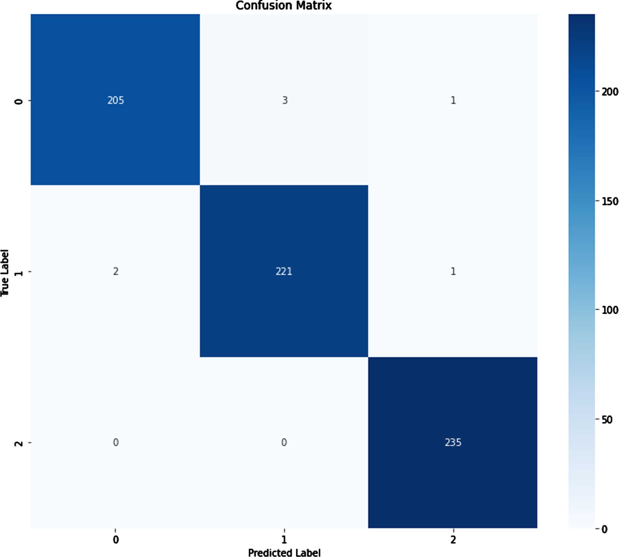
Confusion Matrix of Proposed work.

To back up this claim, the suggested technique is evaluated against a variety of publicly accessible internet datasets. Using the HRF dataset, the suggested model has a 96.15 percent specificity, demonstrating its ability to accurately reject the normal picture.

5 Conclusion

To minimize irreversible structural damage and visual loss, age related macular degeneration must be recognized early. The suggested study’s goal is to create a new optimization-driven strategy-based recurrent neural network for detecting age-related macular degeneration utilizing the Internet of Things. The High-Resolution Fundus (HRF) Image dataset and the MESSIDOR dataset with training data and K-fold are used in this chapter to analyse various approaches. Both 256-pixel and 512-pixel images are used in the study. Additionally, the suggested method’s efficacy is examined by an analysis of its performance in terms of sensitivity, accuracy, and specificity. It is shown analytically that the suggested PSO+RNN enhanced accuracy by 96.194%, sensitivity by 97.184%, and specificity by 97.204%. Based on empirical evidence, it may be concluded that the suggested systems are superior to the state-of-the-art alternatives.

References

Mukai

, Kataoka

, Tanaka

, Miyara

, Maruko

, Nakayama

, Watanabe

, Yamamoto

, Wakatsuki

, Onoe

and Wakugawa

, Three-month outcomes of faricimab loading therapy for wet age-related macular degeneration in Japan, Scientific Reports 13(1) (2023), 8747.

Leung, Ella H., Oh

Daniel J.

, Alderson

Shannon E.

, Bracy

Joshlynn

, McLeod

Mia

, Perez

Litzi I.

, Bottini

Alexander

, Yee

David Chin

and Mukkamala

Krishna

, Initial real-world experience with faricimab in treatment-resistant neovascular age-related macular degeneration, Clinical Ophthalmology (2023), 1287–1293.

Masayuki

Hata

, Hata

Maki

, Andriessen

Elisabeth MMA

, Juneau

Rachel

, Pilon

Frédérique

, Crespo-Garcia

Sergio

, Diaz-Marin

Roberto

et al. Early-life peripheral infections reprogram retinal microglia and aggravate neovascular age-related macular degeneration in later life, The Journal of Clinical Investigation 133(4) (2023).

Desideri

Ferro

, Lorenzo , Traverso

Carlo Enrico

, Nicolò

Massimo

and Munk

Marion R.

, Faricimab for the Treatment of Diabetic Macular Edema and Neovascular Age-Related Macular Degeneration, Pharmaceutics 15(5) (2023), 1413.

Levon

M. Khachigian

, Liew

Gerald

, Teo

Kelvin YC

, Wong

Tien Y.

and Mitchell

Paul

, Emerging therapeutic strategies for unmet need in neovascular age-related macular degeneration, Journal of Translational Medicine 21(1) (2023), 133.

Tan, Yao, Huang

Jianguo

, Li

Deshuang

, Zou

Chang

, Liu

Dongcheng

and Qin

, Single-Cell RNA sequencing in Dissecting Microenvironment of Age-related Macular Degeneration: Challenges and Perspectives, Ageing Research Reviews (2023), 102030.

Gao, Huiqin, Chen

Muchao

, Liu

Yan

, Zhang

Dandan

, Shen

Jingjing

, Ni, Zhimin Tang et al. Injectable Anti-Inflammatory Supramolecular Nanofiber Hydrogel to Promote Anti-VEGF Therapy in Age-Related Macular Degeneration Treatment, Advanced Materials 35(2) (2023), 2204994.

Yue

Tang

, Kang

Yueyue

, Zhang

Xinru

and Cheng

Caiyi

, Mesenchymal stem cell exosomes as nanotherapeutics for dry age-related macular degeneration, Journal of Controlled Release 357 (2023), 356–370.

Xuan

Cao

, Sanchez

Jaron Castillo

, Patel

Tapan P.

, Yang

Zhiyong

, Guo

Chuanyu

, Malik

Danyal

, Sopeyin

Anuoluwapo

, Montaner

Silvia

and Sodhi

Akrit

, Aflibercept more effectively weans patients with neovascular age-related macular degeneration off therapy compared with bevacizumab, The Journal of Clinical Investigation 133(2) (2023).

10.

Khalili

Pour Elias

, Bazvand

Fatemeh

, Iyer

Hassan Kh Siva

, Roohipourmoallai

Ramak

and Hajizadeh

Fedra

, Age-related macular degeneration, Atlas of Ocular Optical Coherence Tomography (2023), 35.

11.

Anisha

Anand

, Jian

Hong-Jyuan

, Huang

Hao-Hsin

, Hean

Li Er

, Li

Yu-Jia

, Lai

Jui-Yang

, Chou

Hung-Da

et al. Anti-angiogenic carbon nanovesicles loaded with bevacizumab for the treatment of age-related macular degeneration, Carbon 201 (2023), 362–370.

12.

de Jong, Sarah, Tang

Jiaqi

and Clark

Simon J.

, Age-related macular degeneration: A disease of extracellular complement amplification, Immunological Reviews 313(1) (2023), 279–297.

13.

Diao, Shengyong, Su

Jinzhu

, Yang

Changqing

, Zhu

Weifang

, Xiang

Dehui

, Chen

Xinjian

, Peng

Qing

and Shi

Fei

, Classification and segmentation of OCT images for age-related macular degeneration based on dual guidance networks, Biomedical Signal Processing and Control 84 (2023), 104810.

14.

Dörschmann, Philipp, Thalenhorst

Tabea

, Seeba

Charlotte

, Tischhöfer

Marie-Theres

, Neupane

Sandesh

, Roider

Johann

, Alban

Susanne

and Klettner

Alexa

, Comparison of Fucoidans from Saccharina latissima Regarding Age-Related Macular Degeneration Relevant Pathomechanisms in Retinal Pigment Epithelium, International Journal of Molecular Sciences 24(9) (2023), 7939.

15.

Bressler, Neil M., Veith

Miroslav

, Hamouz

Jan

, Ernest

Jan

, Zalewski

Dominik

, Studnička

Jan

, Vajas

Attila

et al. Biosimilar SB11 versus reference ranibizumab in neovascular age-related macular degeneration: 1-year phase III randomised clinical trial outcomes, British Journal of Ophthalmology 107(3) (2023), 384–391.

16.

Wei, Wei, Southern

Joshua

, Zhu

Kexuan

, Li

Yefeng

, Cordeiro

Maria Francesca

and Veselkov

Kirill

, Deep learning to detect macular atrophy in wet age-related macular degeneration using optical coherence tomography, Scientific Reports 13(1) (2023), 8296.

17.

Wykoff, Charles C., Brown

David M.

, Reed

Kimberly

, Berliner

Alyson J.

, Gerstenblith

Adam T.

, Breazna

Aurora

, Abraham

Prema

et al. Effect of High-Dose Intravitreal Aflibercept, 8mg, in Patients With Neovascular Age-Related Macular Degeneration: The Phase 2 CANDELA Randomized Clinical Trial, JAMA ophthalmology (2023).

18.

Wykoff, Charles C., Brown

David M.

, Reed

Kimberly

, Berliner

Alyson J.

, Gerstenblith

Adam T.

, Breazna

Aurora

, Abraham

Prema

et al. Effect of High-Dose Intravitreal Aflibercept, 8mg, in Patients With Neovascular Age-Related Macular Degeneration: The Phase 2 CANDELA Randomized Clinical Trial, JAMA ophthalmology (2023).

19.

Shen, Shichen, Kapphahn

Rebecca J.

, Zhang

Ming

, Qian

Shuo

, Montezuma

Sandra R.

, Shang

Peng

, Ferrington

Deborah A.

and Qu

Jun

, Quantitative Proteomics of Human Retinal Pigment Epithelium Reveals Key Regulators for the Pathogenesis of Age-Related Macular Degeneration, International Journal of Molecular Sciences 24(4) (2023), 3252.

20.

Feng, Wei, Duan

Meihan

, Wang

Bingjie

, Du

, Zhao

Yiran

, Wang

Bin

, Zhao

Lin

, Ge

Zongyuan

and Hu

Yuntao

, Automated segmentation of choroidal neovascularization on optical coherence tomography angiography images of neovascular age-related macular degeneration patients based on deep learning, Journal of Big Data 10(1) (2023), 1–11.

Detection and diagnosis of age-related macular degeneration using recurrent neural network with cloud architecture and internet of things

Abstract

Keywords

1 Introduction

2 Related work

3 Proposed methodology

3.2 Image preprocessing

Table 1 Common kernel functions with functional expressions Kernel function name Formula Gaussian K (x i , x j ) = exp(- ∥ x i - x j ) ∥ 2) Linear K (x i , x j ) = x i ′x j Quadratic K (x i , x j ) = (x i , x j + 1) 2 Cubic K (x i , x j ) = (x i ′x j + 1) 3

References

Table 1
Common kernel functions with functional expressions

Kernel function name Formula

Gaussian K (x_i, x_j) = exp(- ∥ x_i - x_j) ∥ ²)

Linear K (x_i, x_j) = x_i^′x_j

Quadratic K (x_i, x_j) = (x_i, x_j + 1) ²

Cubic K (x_i, x_j) = (x_i^′x_j + 1) ³