Pedestrian trajectory prediction method based on automatic driving

Abstract

Pedestrian trajectory prediction plays a crucial role in autonomous driving, as its accuracy directly affects the autonomous driving system’s comprehension of the environment and subsequent decision-making processes. Current trajectory prediction methods tend to oversimplify pedestrians to mere point coordinates, utilizing positional information to infer interactions among individuals while overlooking the temporal correlations between them, thereby excessively simplifying pedestrian characteristics. To address the aforementioned issues, this paper proposes a trajectory prediction model for autonomous driving applications, that takes into account both pedestrian motion characteristics and scene interaction. The model optimizes the LSTM unit structure twice, serving to learn correlations among long trajectories of pedestrians and to integrate multiple forms of information into the neighborhood interaction module. Furthermore, our model introduces dual attention mechanisms for individuals and scenes, focusing on the key motion points of individual pedestrians and their interactive behavior with others in busy scenarios. The efficacy of the model was validated on the MOT16 pedestrian dataset and the Daimler pedestrian path prediction dataset, outperforming mainstream methods with 8% and 10% reductions in Average Displacement Error and Final Displacement Error respectively.

Keywords

Trajectory prediction automated driving CNN-LSTM deep learning

1 Introduction

As autonomous driving technology continues to advance, pedestrian trajectory prediction has become a critical component in the domain of autonomous driving [1]. Its primary objective is to forecast the future positions of individuals. The growing complexity of modern traffic scenarios heightens the risk of accidents driven by delayed driver reactions or inaccurate judgements regarding pedestrian movements on the streets. Pedestrian trajectory prediction methods, when deployed in autonomous driving systems, are capable of making swift and precise decisions [2], significantly enhancing the safety performance and decision-making of self-driving vehicles. Consequently, accurately predicting pedestrian future location information bears great significance. Autonomous vehicles need to accurately anticipate future pedestrian trajectories to improve their predictive capabilities regarding road conditions, thereby enhancing road safety.

Predicting pedestrian group trajectories in complex traffic scenarios remains a challenging task. The difficulty lies in addressing issues such as diversity, dynamics, and temporal dependence of trajectories [3]. Pedestrian behavior diversity stems from individual habits and social norms. Dynamics indicate the variability of pedestrian behavior with environmental changes. Moreover, pedestrian actions exhibit temporal dependency, potentially influenced by past behavior. Although predicting individual behavior poses challenges, advanced machine learning algorithms have made significant strides in handling these uncertainties. Topal et al. [19] have contributed to autonomous vehicle technology by detecting vehicles using FR-CNN and drawing lane lines with Canny edge detection and Hough transform, where such positional data are used to assess driver intent and prevent potential accidents. However, trajectory prediction in the context of autonomous driving requires consideration of additional pedestrian and environmental factors, such as speed, walking direction, intent, and interpersonal relations. Furthermore, pedestrians typically do not make decisions in isolation but must consider interactions with nearby vehicles and other pedestrians.

Figure 1 illustrates the influence of different information factors on predicting pedestrian trajectory in traffic scenarios. For agent 1, Fig. 1(a) shows the trajectory prediction using only historical pedestrian data (historical trajectory and size of the pedestrian). Figure 1(b) includes both pedestrian history and vehicle motion in predicting the future trajectory. In addition to historical and vehicle motion data, Fig. 1(c) also considers agent 1’s head direction, indicating intent. Experimental results demonstrate that the prediction in Fig. 1(c) is the closest to the actual scenario, achieving the smallest error. Thus, incorporating additional information factors, such as head direction and vehicle data, is crucial for improving prediction accuracy.

Fig. 1

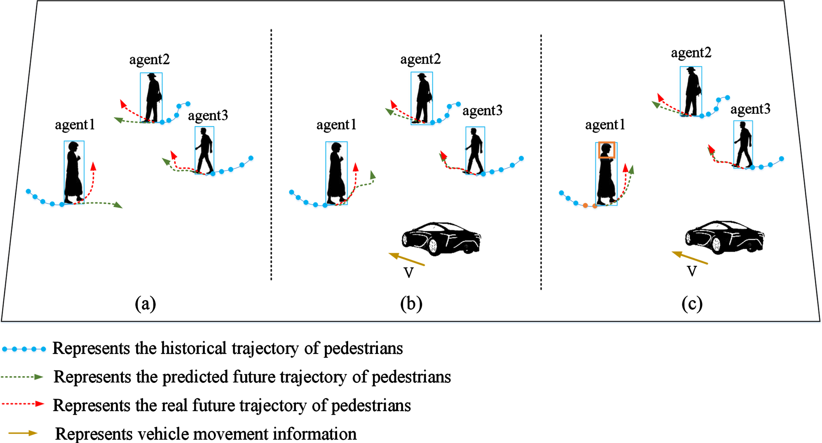
Historical trajectory and future trajectory of the agent in different scenarios.

Current pedestrian trajectory prediction methodologies predominantly rely on pedestrian positional data [4–6], which often inadequately leverage pedestrian and contextual scene information, failing to integrate pedestrian dynamics with the spatial-temporal context. Therefore, it is imperative to delve into this area for more effective predictive frameworks. This article introduces the SGPN trajectory prediction model that amalgamates CNN and LSTM with a dual-attention mechanism to holistically encapsulate individual pedestrian attributes and the pertinent environmental cues for future path estimation. The model specifically accounts for individual pedestrian information, such as historical trajectories and physical dimensions, head pose data, and contextual scene details, including interactions with proximate pedestrians and vehicles. SGPN optimizes the LSTM for individual pedestrian feature representation as well as group interaction, introduces a dual attention mechanism to highlight key motion information, resets the neighborhood, and incorporates the pedestrian’s head direction and speed vector into the interaction module. This approach caters to both the temporal feature information of individual pedestrians and the spatial interaction information of neighboring pedestrians from the driver’s perspective. The main contributions of this paper are as follows:

1. Addressing the discrepancy between vehicular perspective and actual three-dimensional spatial distances by proposing a predictive module that combines multiple feature information sources. This module learns from pedestrian trajectories and size, considering the impact of pedestrians’ head intention data and the vehicle’s own motion information.

2. Acknowledging the dual impact of individual features and group interaction on trajectory prediction, the Motion Feature Module and Scene Interaction Module are employed to achieve integration of information in both temporal and spatial domains. The Motion Feature Module uses a Tree-LSTM [7] structure to document pedestrian feature information at different times. The Scene Interaction Module addresses spatial interaction issues amongst nearby pedestrians.

3. To focus on the key movement of pedestrians and key spatial interaction information, self-attention mechanism and scene attention mechanism are respectively introduced to strengthen the model’s ability to learn the key information.

2 Related work

2.1 Pedestrian trajectory prediction method based on shallow learning

Early trajectory prediction techniques involved coupling elementary kinematic models (constant velocity/acceleration/turning), Probabilistic models [13], and Bayesian filters [8] or their extensions to anticipate the future positions of pedestrians. Helbing and Molanari [9] proposed a social force model based on Newtonian Mechanics, a method that has proven effective for predicting pedestrian trajectories. However, relying solely on manually designed features makes it difficult to capture interactive behaviors in complex scenarios. Schneider et al. [10] carried out a comparison between singular Kinematic model and multi-model-based approaches, which, while reducing location errors, was at odds with reality as it assumed constant speed. Pavlovi et al. [11] developed the Switched Linear Dynamical System (SLDS) model, a Markov chain-based probability transition model utilizing multiple linear motion model switching for predicting actual non-linear motion. The drawback is, this model relies on switching between movement characteristics of different states, falling short in scenarios involving multifaceted and interwoven mathematical descriptions. Bhaskara et al. [12] introduced a novel trajectory prediction model dubbed FlowMNO, which integrates a Markov process with optical flow as a pivotal component, delivering fresh perspectives within pedestrian path forecasting.

2.2 Pedestrian trajectory prediction method based on deep learning

Unlike shallow learning, deep learning does not require an established mathematical model. Instead, the network can learn sensible mapping relationships through large-scale datasets. With the recent advancements in deep learning, a wide range of models for processing temporal data have been proposed, making neural network-based trajectory prediction algorithms [14–16] mainstream, delivering significantly improved results in comparison to traditional algorithms.

Recurrent Neural Networks (RNN) [17], including variants such as LSTM and Gated Recurrent Unit (GRU) [18], have yielded significant results in trajectory prediction tasks [20]. Alahi et al. [22] first proposed the Social LSTM (S-LSTM) for trajectory prediction. This data-driven deep learning method achieved promising results on public datasets like ETH [23] and UCY [24]. Inspired by this, many have pursued similar research, the Group LSTM (G-LSTM) [26], an improved method of S-LSTM, leverages motion consistency to gather trajectories with similar motion trends and group pedestrians. However, the presumption of S-LSTM and G-LSTM that individual influences are determined by their locations is overly simplistic and cannot reflect the realities of traffic scenarios. Recently, Rashmi et al. [25] proposed the Social Group LSTM model (SG-LSTM), utilizing group dynamics for pedestrian trajectory prediction, but it only functions within short distances and disregards environmental information. Finally, Takuma Yagi et al. [33] used CNN to extract pedestrian and environment information and integrate them, proposing the FPL network model, which demonstrated impressive prediction results. The standalone application of CNN networks faces challenges in attending to the temporal and spatial sequence data of pedestrian motion, resulting in constrained predictive power for complex traffic contexts.

Addressing these limitations, we propose the SGPN model. The significant departure from previous research lies in our model’s integration of pedestrian characteristics with environmental information. It adeptly combines pedestrian features and group interactions into a cohesive framework and assigns tailored attention mechanisms to each module, thereby facilitating a more comprehensive understanding of the scene and decision-making process. Consequently, this enables a more effective prediction of pedestrian future trajectories.

3 Problem definition

The pedestrian trajectory prediction problem is defined as follows: predicting the trajectory of the target pedestrian i (i ∈ N, N represents the set of all pedestrians in the scene) at time t. At this time, all the feature information of the target pedestrian i can be denoted as $A_{t}^{i}$ . Here, t₀ - T_his represents the time point when the pedestrian is first observed, t₀ represents the current moment and t₀ + T_future represents the final frame of the trajectory prediction for the pedestrian. Thus, the time interval [t₀ - T_his, t₀] represents the observation period for pedestrian i. The input of the historical features is represented as $A^{i} = Σ_{t = t_{0} - T_{his}}^{t_{0}} A_{t}^{i}$ . Given Aⁱ, the trajectory prediction module generates the future trajectory Zⁱ of pedestrian i in the time span [t₀, t₀ + T_future].

In our methodology, a pedestrian’s current state is determined by features encompassing their historical trajectory, dimensions, speed, and head direction. The predicted location is realized through our model, which takes the pedestrian’s existing state as input. Initially processed by Feature Fusion Module, the input is then subjected to trajectory forecasting by our prediction module, yielding the most precise prediction of position. It is imperative to emphasize that the process of decision-making for each action does not rely on traditional methods, such as Q-learning or policy iteration; instead, it is accomplished through the deep learning model SGPN designed in this study. These concepts will be elaborated upon in Section 4, dedicated to explicating the operational principles and implementation specifics of SGPN.

4 The proposed model

SGPN focuses on the individual pedestrian’s characteristics and interactions within the crowd. The overall network prediction framework is presented in Fig. 2. Specifically, the SGPN is composed of five modules: the Feature Fusion Module (FFM), the Motion Feature Module (MFM), the Scene Interaction Module (SIM), the Dual Attention Mechanism (DAM) and the Decoding Function Module (DFM). From Subsection 4.1 to 4.4, we elaborate on the features and functions of each module, as well as how they interact towards the goal of predicting pedestrian trajectories. A detailed description of the SGPN framework follows:

Fig. 2

General overview of the SGPN model.

Initially, our SGPN model extracts key information from observed motion sequences of pedestrians and vehicles, including position, velocity, and direction. This information is then fused into a sequence of length A^N via a one-dimensional fully convolution network, serving as input for the subsequent prediction module. Furthermore, we employ an enhanced Tree-LSTM as our principal information updating framework, which utilizes contextual data to more precisely capture pedestrian characteristics. The model assigns variable weights to individual pedestrian features and constructs feature outputs based on the significance of the outputted hidden states. Subsequently, the updated sequential information is processed by the SIM, which captures the complex spatial interactions between pedestrians, and between pedestrians and vehicles, through an elliptical neighborhood matrix. Our work specially designs a dual attention mechanism comprising both an intrinsic attention, focusing on the internal state changes of the pedestrians, and a contextual attention, dedicated to capturing detailed interactions between pedestrians and their surrounding environment. This enables the model to identify and emphasize important features. Lastly, the prediction module concatenates the encoder’s final hidden features with the latent variable z and generates the motion prediction sequence Z^N through an LSTM decoder.

4.1 Feature Fusion Module (FFM)

The objective of this study is to predict future pedestrian positions. Towards this goal, multiple influential factors need to be considered. Firstly, a pedestrian’s historical trajectory serves as a crucial determinant of their future positions. Given the inconsistency between the perspective distance in the shooting video and the actual physical space, we adopt a joint learning approach to process the information of the pedestrian’s trajectory and size. Additionally, the status of a vehicle could influence a pedestrian’s route. Therefore, we employ an egomotion algorithm to capture the vehicle’s self-movement. Lastly, to gain a more refined understanding of pedestrian movement, we incorporate information about the pedestrian’s head direction. This data is encoded and included in our analysis, the details of which will be explained later.

We perform joint learning on pedestrian position and size to mitigate the influence of perspective effect. Initially, we preprocessed the input video sequences to obtain the position coordinate information $(x_{t}^{i}, y_{t}^{i})$ (where $(x_{t}^{i}, y_{t}^{i}) \in R_{+}^{2}$ represents the two-dimensional coordinates of the pedestrian at time t) and size $s_{t}^{i}$ (where s_t ∈ R₊) of the target pedestrian i at time t. The joint learning of these two parameters can yield the coordinate and size information of pedestrian i at time t, denoted as $m_{t}^{i} = {((x_{t}^{i}, y_{t}^{i})^{T}, s_{t}^{i})}^{T}$ .

Pedestrians may have to adjust their walking routes due to the movement of a driving car, especially when the vehicle is in close proximity, to avoid potential collisions. To enhance the positioning performance of the first-person perspective videos, we have utilized the egomotion algorithm to acquire the vehicle’s self-motion information. We can get t under the moment of rotation matrix r_t (ψ, ∅ , θ) and translation vector v_t (v_x, v_y, v_z), vehicle since the movement information is expressed as e_t = (r_t^T, v_t^T) ∈ R⁶.

The direction in which a pedestrian’s head is positioned can specifically indicate their movement direction. The head direction is defined using head rotation angles with values ranging from ωϵ (0, 360°). Hence, the head direction problem can be treated as a classification-regression problem. The method of Histograms of Oriented Gradients (HOG) and Support Vector Machine (SVM) is used to divide a pedestrian’s head into eight directions, represented as 0–7, where the head direction differs by 45° between two adjacent categories. First, the HOG feature describing pixel intensity gradients is applied, followed by the SVM classification method. If the pedestrian’s head image at time t is represented as p_t, where d = 0, 1, … 7, then the probability of head direction can be expressed as follows: $p_{t} = SVM (HOG (d))$ (1)

Fig. 3

Head direction classification.

In the FFM module, the overall feature information,

A_{t}^{i}

, of the target pedestrian i at time t can be expressed as follows:

A_{t}^{i} = (m_{t}^{i}, e_{t}, p_{t}^{i})^{T}

(2)

The network architecture of FFM is depicted in Table 1. The input dimensions, denoted as D, vary for each stream. For instance, D = 3 for the position-scale stream, D = 6 for the egomotion stream, and D = 1 for the head direction. A fully convolutional network, equipped with four One-Dimensional (1D) convolution filters, processes the data feature series, each followed by a ReLU activation function and a Batch Normalization (BN) layer. This design augments the non-linearity of the network model, stabilizes training, accelerates convergence, and reaps better results. The position scale information, vehicle self-motion information and pedestrian head information were respectively obtained by four-layer convolution neural network to obtain 128 × 2 historical feature vectors, which were denoted as M_in, E_in, P_in. By concatenating these three historical feature vectors end to end, the total input feature vector A^N with a size of 384 × 2 is obtained. The total feature vector is put into the subsequent prediction module for further processing.

Table 1

Feature fusion network framework of FFM

Layer type	Channel	Kernel size	Output size
input	-	-	D × 10
1D-Conv+Relu+BN	32	3	32 × 8
1D-Conv+Relu+BN	64	3	64 × 6
1D-Conv+Relu+BN	128	3	128 × 4
1D-Conv+Relu+BN	128	3	128 × 2

4.2 Motion Feature Module (MFM)

The MFM introduced in this study is designed to process a plethora of feature information from the FFM, thereby enhancing the model’s capability to represent pedestrian characteristics through effective information assimilation. Within the MFM, a Tree-LSTM structure is employed to handle diverse feature information in parallel, substantially improving processing efficiency. During each iteration, the feature queue is updated by incorporating the latest frame’s characteristics, ensuring continuous refinement of pedestrian feature representation.

To overcome the limitations of traditional LSTM models in learning long-term dependencies, this study employs a Tree-LSTM structure to enhance the modeling capability for complex, long-duration sequential data. Unlike LSTM models which process information in a sequential manner, the Tree-LSTM leverages its hierarchical structure to process and optimize multiple input features in parallel, rendering it more adept at capturing intricate and prolonged temporal correlations, thus boosting efficiency and model performance. In this study, the Tree-LSTM model has been refined, assigning variable weights to the feature information of individual pedestrians. These weights are predicated on the significance of the output hidden states, formulating a tailored feature module for each pedestrian.

In the MFM, the latest frame’s features are added to the queue to update it in each iteration within the features information from FFM transferred to the Tree-LSTM unit. Multiple forget gates are used to control the flow of frame information in the queue. If a pedestrian’s motion exhibits instability or discontinuity in temporal continuity with historical states, the self-adjusting ability of Tree-LSTM’s adaptive forget gate becomes crucial, Tree-LSTM can automatically adjust the degree of forget gate opening according to the input information. Consider the historical state [t₀ - T_his, t₀] as a substate of the current state time t₀. We first calculate the sub-state hidden in the final frame’s overall characteristics, this is represented by the formula ${\tilde{h}}_{t}^{i} = Σ_{l = 0}^{T_{his}} h_{t - l}^{i}$ . A special embedding function is used to the information of pedestrian i at time t as a vector, denoted as $a_{t}^{i}$ , the formula is expressed as follows: $a_{t}^{i} = φ_{a} (A^{N}; W_{a}, b_{a})$ (3)

Where φ_a is a multi-layer perceptron with the ReLU activation function. W_a represents the weight matrix of φ_a, and b_a represents its bias matrix. The cell structure diagram of MFM is shown in Fig. 4, and the calculation formula is as follows: $u_{t}^{i} = σ (w_{uh} {\tilde{h}}_{t - 1}^{i} + w_{ua} a_{t}^{i} + b_{u})$ (4) $f_{tl}^{i} = σ (w_{fh} h_{t - 1}^{i} + w_{fa} a_{t}^{i} + b_{f})$ (5) $o_{t}^{i} = σ (w_{dh} {\tilde{h}}_{t - 1}^{i} + w_{da} a_{t}^{i} + b_{d})$ (6) ${\bar{C}}_{t}^{i} = \tanh (w_{ch} {\tilde{h}}_{t - 1}^{i} + w_{ca} a_{t}^{i} + b_{c})$ (7) $C_{t}^{i} = u_{t}^{i} ⊙ {\bar{C}}_{t}^{i} + Σ_{l = 1}^{T_{his}} f_{t}^{il} ⊙ C_{t - l}^{i}$ (8) $h_{t}^{i} = o_{t}^{i} ⊙ \tanh (C_{t}^{i})$ (9)

Fig. 4

The structure of Tree-LSTM.

Among them, the sigmoid function is denoted as σ, $u_{t}^{i}$ , $f_{t}^{i}$ , $o_{t}^{i}$ respectively represent the input gate, the forget gate and the output gate at time t. ⊙ is the product of the corresponding elements, that is, the multiplication of the elements. ${\bar{C}}_{t}^{i}, C_{t}^{i}, h_{t}^{i}$ represent the cell candidate state, the cell state, and the hidden state at time t, respectively. Instead of employing a solitary forget gate, the Tree-LSTM unit encompasses an individual forget gate f_tl for each child l. This allows the Tree-LSTM unit to selectively incorporate information from each child. When T_his = 0, the MFM degenerates into an ordinary LSTM unit, which only considers the characteristics of the t₀ frame in one iteration.

This study builds upon the foundation of the Tree-LSTM model, enhancing its capability to process multiple features. A Tree-LSTM based feature extraction is utilized for each pedestrian, and a weighted construction of individual pedestrian feature modules is facilitated according to varying levels of importance of the hidden states output by the Tree-LSTM. The structure diagram of MFM is shown in Fig. 5, and the specific construction process is as follows:

Following feature fusion via the FFM, the sequence A^N = (a₀, …, a_t) is forwarded to the Tree-LSTM for further processing.

The Tree-LSTM model structure yields a sequence of hidden state outputs h_i = (h₀, …, h_t).

Weights are applied to all hidden states at each input time step, transforming them into outputs at different time points. The corresponding distribution α_i, for i ∈ [0, t], is then determined based on the comparative effectiveness of those states. The calculation formula for α_i is expressed as: $α_{i} = \frac{\exp (score (\bar{h}, h_{i}))}{Σ_{i = 0}^{t} \exp (score (\bar{h}, h_{i}))}$ (10) where score( $\bar{h}$ , h_i) is a scoring function indicative of the extent of attention bestowed upon a pedestrian’s state at any given moment within a defined period. This function elucidates the relative contribution of that moment’s hidden state to the final contextual information representation U_P. The scoring function is computed as follows: $score (\bar{h}, h_{i}) = w^{T} tanh (w_{1} \bar{h} + w_{2} h_{i} + b)$ (11)

Through the computation facilitated by the MFM, pedestrain i’s weighted feature information at each moment from time 0 to t is calculated as $h_{0}^{i}$ = α₀h₀, …, $h_{t}^{i} = α_{t} h_{t}$ . Consequently, the contextual information representation U_p for the pedestrian is obtained. The expression for U_P can be formalized as follows: $U_{P} = (h_{0}^{i}, \dots, h_{t}^{i})$ (12) Subsequently, U_p is passed to the SIM for the processing of information between groups.

Fig. 5

The structure of MFM.

4.3 Scene Interaction Module (SIM)

The SIM is utilized to simulate the motion variations of pedestrians during locomotion, which arise due to environmental factors and interactions with other pedestrians. SIM defines the vicinity of an agent, factoring in the pedestrian’s position, velocity and head orientation to characterize the interactive effects with their neighbors. Upon acquiring information on neighborhood interactions and spatial attention vectors, SIM inputs these into an LSTM network, resulting in updated cell states and hidden states.

A pedestrian’s trajectory within a crowd is heavily influenced by the behaviors of others and environmental conditions. Different people can have varying degrees of impact on one’s movement, even when they share the same pedestrian distance. This is due to individual differences, the mutual influence between two pedestrians who are facing each other in close proximity can be significantly stronger than two passing by back-to-back. This suggests that pedestrian interactions are not only dependent on distance but also on factors such as orientation and walking direction. Combine the above factors, in the SIM, we have refined our scene interaction module, redesigning it to include features that more accurately represent the factors influencing future pedestrian trajectories.

In contrast to existing research on rectangular grid maps, which identify an agent’s neighborhood as a m × n grid parallel to the absolute coordinate axis without considering the direction of the agent’s movement, our study adopts a unique approach. We establish an elliptical neighborhood matrix N₀ for each pedestrian, encapsulating their positional coordinates, velocity data and heading details. This novel methodology ensures a more comprehensive and accurate analysis of pedestrian dynamics.

In defining the neighborhood of an agent, occupancy grid maps are customarily employed, with rectangular and circular grid maps centered on the agent’s current position being particularly prevalent. Figure 6(a) illustrates a typical rectangular grid map, where the grid always runs parallel to the x and y axes, regardless of the agent’s movement direction. There’s a standard assumption that pedestrians distribute their attention evenly across all directions within their neighborhood. However, the agent’s field of vision tends to be broader in the direction of travel, often resulting in greater attention to neighbors upfront and an extended visible range. Contrarily, the rear neighborhood’s impact on the agent is lesser, reciprocally reducing the agent’s rearward focus. Hence, to capture more holistically in the model how a neighbor might influence an agent’s future trajectory, we introduce the concept of anisotropic neighborhoods after conducting a coordinate transformation. As depicted in Fig. 6(b), such neighborhood settings yield neighborhoods in front and behind the agent symmetric to the y - axis, making it more representative of an agent’s perceptual reality. The neighborhood N₀ is defined as: $\frac{{(y - \frac{a}{2})}^{2}}{a^{2}} + \frac{x^{2}}{b^{2}} = 1$ (13)

Fig. 6

Neighborhood size definition. (a) Rectangular grid map neighborhood; (b) This paper presents the elliptic graph neighborhood.

Among them, (x, y) are points in relative coordinates. a, b are parameters that define the neighborhood, where a > b > 0. The Y - axis of the neighborhood is consistent with the speed direction of the pedestrian at the current moment, and the neighborhood design simulates the attention of the pedestrian in the actual walking process.

Velocity, head information and position information are used to model interactions among pedestrians. By integrating the cell states of surrounding pedestrians from the previous moment, the interactive scenario within a pedestrian’s neighborhood at time t is obtained. This is designated as the neighborhood pedestrian information sharing module, denoted as $N_{t}^{i}$ , as illustrated in formula (14). $N_{t}^{i} = Σ_{j \in N_{i}} ({\bar{v}}_{t}^{i, j}, d_{t}^{i, j}, {\bar{p}}_{t}^{i, j}) | h_{t - 1}^{j}, c_{t - 1}^{j}$ (14)

Among them, N_i refers to the ith individual corresponding neighborhood set, and j is the pedestrian in the neighborhood corresponding to N_i, j ≠ i. ${\bar{v}}_{t}^{i, j}$ represents the relative speed of the pedestrian in the neighborhood and the target pedestrian; $d_{t}^{i, j}$ represents the direction of the head of the pedestrian in the neighborhood and the target pedestrian; ${\bar{p}}_{t}^{i, j}$ represents the relative position and angle between the neighborhood pedestrian and the target pedestrian, where ${\bar{p}}_{t}^{i, j} = (x_{t}^{j} - x_{t}^{i}, y_{t}^{j} - y_{t}^{i}) arctan \frac{y_{t}^{j} - y_{t}^{i}}{x_{t}^{j} - x_{t}^{i}}$ . $h_{t - 1}^{j}$ and $c_{t - 1}^{j}$ correspond to the hidden state and cell state of LSTM corresponding to individual jth at time t - 1, respectively.

Put $N_{t}^{i}$ into the input end of the LSTM network to get the new cell candidate state of the SIM module ${\tilde{C}}_{t}^{i}$ : ${\tilde{C}}_{t}^{i} = C_{t}^{i} + \tanh (W_{c} (N_{t}^{i} + L_{t}^{i, j}))$ (15)

Where $L_{t}^{i, j}$ represents the spatial attention vector in the scene interaction, which we cover in detail in the DAM. The cell state $C_{t}^{'}$ and the hidden state $h_{t}^{'}$ of the SIM module are expressed as follows: $C_{t}^{'} = f_{t} C_{t - 1} + i_{t} {\tilde{C}}_{t}^{i}$ (16) $h_{t}^{'} = o_{t} \tanh (C_{t}^{'})$ (17) The LSTM structure of the SIM is shown in Fig. 7.

Fig. 7

The structure of SIM.

4.4 Dual Attention Mechanism (DAM)

The DAM is designed to enhance focus on salient information regarding both pedestrians and the environment, thus refining the accuracy of pedestrian trajectory prediction. Tailored to the distinct characteristics of the MFM and SIM modules, an intrinsic self-attention and an extrinsic scene attention mechanism have been implemented. The self-attention mechanism correlates the historical motion states of pedestrians to capture individual behavior traits, enabling the model to concentrate on pivotal movement patterns. Conversely, the scene attention mechanism delves into the analysis of interactions between pedestrians and their surroundings, scrutinizing the influence of neighboring pedestrian dynamics on a target individual’s state.

When pedestrians are walking, their attention is mainly focused on the road conditions ahead, surrounding pedestrians and vehicles, and other potential hazards. This involves the brain’s filtering of important information and the allocation of attention to ensure that pedestrians can safely and efficiently reach their destinations. In pedestrian trajectory prediction models, introducing a self-attention mechanism first extracts information from the FFM, associates the pedestrian’s historical motion states, and approaches from a temporal perspective, enabling the model to learn how to focus on the key points of pedestrian movement.

We extract $h_{t}^{i}$ from all observed time steps in Tree-LSTM and concatenate it into the feature tensor Hⁱ for the target pedestrian i, denoted as $H^{i} = (h_{t_{0} - T_{his}}^{i}, . . ., h_{t_{0}}^{i})$ . To establish the connection between the current moment and the past moments for a pedestrian, we introduce the self-relation parameter tensor Kⁱ, which can be represented as: $K^{i} = φ_{k} (u_{t - 1}^{i}, h_{t_{0}}^{i}; W_{k})$ (18)

Among them, φ_k (·) denotes a multi-layer perceptron with ReLU as the activation function and W_k represents its weight matrix. Kⁱ represents the intrinsic dynamic relationship of changes in the motion state of pedestrian i from time t₀ - 1 to t₀. It is a quantitative measure of the relationship between the current behavioral state and past behavioral state, aiding the network’s understanding and learning of pedestrian movement characteristics. The larger the value of Kⁱ, the more it indicates that the movement state of pedestrian i has maintained a high level of continuity from time t - 1 to t. Additionally, the network sets up an independent self-attention mechanism for each pedestrian in the scene, and the score of i’s self-attention mechanism at time t can be expressed as follows: $α_{t}^{i} = Softmax ({Score}_{α} (H^{i}, K^{i}))$ (19)

Among them, Score_α (·) is the scoring function of this module. Since pedestrians are local elements in the scene, local attention employs the conventional scoring function, as shown in the formula (20): ${Score}_{α} (H^{i}, K^{i}) = W_{α} (H^{i})^{T} K^{i}$ (20)

Where, W_a is the weight parameter matrix of the regular scoring function. At this point, we add the product of the self-attention score and the hidden state of pedestrian i to obtain the context propagation vector Gⁱ of this module: $G^{i} = Σ_{t = 0}^{t_{0}} α_{t}^{i} h_{t}^{i}$ (21)

To describe scene information in more detail, we introduced a scene attention mechanism. This measure aims to avoid the problems of insufficient scene description and inadequate description of pedestrian status caused by a single attention mechanism. It further enhances the accuracy of pedestrian trajectory prediction. The participants walking in the scene constitute the scene information. To describe the influence of interactions between pedestrians on the target pedestrian’s state, we introduce the spatial attention vector $L_{t}^{i, j}$ . First, we process the scene information to obtain the relative spatial state $l_{t}^{i, j}$ :

$l_{t}^{i, j} = φ_{l} (N_{t}^{i, j}; W_{l})$ (22)

Among them, φ_l (·) Representing a multi-layer perceptron with ReLU as the activation function, and W_l as the weight parameter matrix for φ_L. Where, $N_{t}^{i, j}$ represents the scene information of target pedestrians and other pedestrians in the neighborhood, with i ≠ j. Based on the relationship between the relative spatial state $l_{t}^{i, j}$ and the context transmission vector G^j of the neighboring pedestrians in the scene, we can obtain the attention score $β_{t}^{i}$ of the target pedestrian i towards the other pedestrians in the neighborhood. The equation is expressed as:

$β_{t}^{i} = Softmax ({Score}_{β} (l_{t}^{i, j}, G^{j}))$ (23)

Score_β is the scoring function of this module. In the SIM, what is calculated is the attention of the target pedestrian i to all pedestrians in the scene. Dot multiplication intuitively reflects the similarity between pedestrians, hence the scene attention mechanism employs point multiplication for scoring, as shown in formula (24). ${Score}_{β} (l_{t}^{i, j}, G_{t}^{j}) = l_{t}^{i, j} G_{t}^{j}$ (24)

By accumulating the product of the scene attention score and the context propagation vector of all other pedestrians j in the neighborhood, we can obtain the scene attention vector $L_{t}^{i, j}$ : $L_{t}^{i, j} = Σ_{t = 0}^{t_{0}} β_{t}^{i, j} C^{j}$ (25) The structure of the DAM module is shown in Fig. 8:

Fig. 8

The structure of DAM.

We connect the last hidden feature in the encoder with the latent variable to predict motion through the LSTM decoder.

5 Experimental setting

In this section, we have introduced the experimental datasets, experimental environment, evaluation metrics, and parameter settings. Subsequently, we conducted cross-validation experiments, ablation experiments, and model training. Cross-validation experiments for model performance evaluation and generalization ability estimation, ablation experiments to help understand the functions of various components of the model, and model training through parameter adjustment and optimization to enhance model prediction accuracy, constitute major processes in validating the efficacy of the model and exploring the performance thereof.

5.1 Dataset description

The datasets used in this experiment are pedestrian video datasets shot from a first-person perspective: The Daimler Pedestrian Path Prediction Benchmark Dataset [28] and the MOT16 pedestrian dataset [29].

Daimler Pedestrian Path Prediction Benchmark Dataset (Daimler dataset). Dataset includes 68 videos of pedestrians in, captured using stationary and moving vehicles. Vehicle sensors recorded speed and lateral acceleration to represent self-motion The dataset considered four different types of pedestrian motion: bending in, stopping, crossing, and starting. The scenes captured ranged in complexity, from streets to parks to commercial centers, covering a variety realistic and complex scenarios. Figure 9 shows examples of different scenes captured in the Daimler dataset, a, b, c, d representing the four different types of pedestrian motion.

Fig. 9

The shooting frames of Daimler dataset under different scenes.

MOT16 pedestrian dataset. As part of the MOT Challenge introduced in 2016, the MOT16 pedestrian dataset features 14 videos of various pedestrian motions, including camera calibration details for each frame. The dataset consists of 7 different scenes, capturing various pedestrian motions and backgrounds. It has become a standard dataset for evaluating and validating multiple object tracking algorithms, with many research achievements building upon it. Two videos, MOT16-13-raw and MOT16-14-raw, which were not captured from a first-person perspective, were excluded from our experiment.

5.2 Setting of experimental environment and parameters

The configuration of the experimental environment in this study includes Windows 10 operating system, an Inter Xeon E5-2620 v4 CPU, and an NVIDIA GeForce RTX 2080Ti GPU. The experiment was carried out in the Python programming language with PyTorch 1.7.1 serving as the deep learning framework, and CUDA version 11.0 for building our network model training.

Overfitting is one of the common issues encountered when training deep learning models; at its core, it stems from the model excessively focusing on the details within the training set, thereby neglecting the true patterns and structures. To mitigate this problem, the present study employs L2 regularization. The training of the model utilized the Adam optimization algorithm, which integrates the advantages of momentum and adaptive gradient methods. It adjusts the learning rate by updating both the first-order and second-order moment estimates, thereby enabling more efficient parameter updates. The computational formula for the Adam algorithm is as follows: $g_{t} = \frac{\partial L}{\partial W_{t}}$ (26) $m_{t} = β_{1} m_{t - 1} + (1 - β_{1}) g_{t}$ (27) $v_{t} = β_{2} v_{t - 1} + (1 - β_{2}) g_{t}^{2}$ (28) ${\hat{m}}_{t} = \frac{m_{t}}{1 - β_{1}}$ (29) ${\hat{v}}_{t} = \frac{v_{t}}{1 - β_{2}}$ (30) $W_{t + 1} = W_{t} - \frac{η {\hat{m}}_{t}}{\sqrt{{\hat{v}}_{t} + ϵ}}$ (31)

Where m_t and v_t represent the estimates of the first and second moments, respectively; β₁ and β₂ are hyperparameters that control the exponential decay rates for these moment estimates; ${\hat{m}}_{t}$ and $\hat{v} t$ are the bias-corrected estimates of the first and second moments; W_t+1 denotes the updated parameters; η is the learning rate, and ϵ is a small positive constant for numerical stability. This approach facilitates the navigation of the parameter space, potentially leading to a more swift convergence towards the optimal solution.

The initial learning rate of the model was set to 0.001 with hyperparameters β₁= 0.9, β₂ = 0.999, and a regularization coefficient of 0.001. The batch size was designated as 64, and the momentum was configured to 0.99. A total of 200 iterations were planned for the training of the model. To further enhance the model’s performance, a learning rate scheduling strategy was implemented: the learning rate was scaled down by a factor of 0.5 and 0.1 upon reaching the 50th and 150th training epochs, respectively. This adjustment technique assists in extricating the model from local minima and steering it towards the global optimum. Observations from our experimental outcomes indicate that such modifications significantly augment the model’s rate of convergence and its eventual performance.

5.3 Evaluation metrics

In order to evaluate the performance of the proposed model, the evaluation indexes commonly used in trajectory prediction research were adopted in this paper: Average Displacement Error (ADE) and Final Displacement Error (FDE).

ADE: In trajectory prediction, the average value of the predicted position at each moment and the Euclidean distance corresponding to the true trajectory position. The calculation process is shown in formula (32): $ADE = \frac{Σ_{i = 1}^{N} Σ_{t = t_{0} + 1}^{t_{0} + T} \sqrt{{({\bar{x}}_{i} - x_{i})}^{2} + {({\bar{y}}_{i} - y_{i})}^{2}}}{NT}$ (32) $({\bar{x}}_{i}, {\bar{y}}_{i})$ represents the pedestrian actual coordinates, every moment (x_i, y_i) pedestrian prediction coordinates every moment, N indicates the total number of pedestrians for trajectory prediction.

FDE: In trajectory prediction, the Euclidean distance between the predicted position of the final trajectory and the real final destination. The calculation process is shown in formula (33): $FDE = \frac{Σ_{i = 1}^{N} \sqrt{{(\bar{x} - x)}^{2} + {(\bar{y} - y)}^{2}}}{N}$ (33) $(\bar{x}, \bar{y})$ represents the pedestrian final location of the actual coordinates, (x, y) pedestrian final location prediction coordinates.

5.4 Cross-validation experiment

The training and validation dataset were randomly divided in a 4:1 ratio, followed by cross-validation experiments to validate the performance of the proposed model and to assess it. The evolution of the model’s training loss function value on the dataset is depicted in Fig. 10. Each set of cross-validation experiments were executed through 200 epochs. The five differently colored curves in the figure represent the changes in the training loss function value for the five cross-validation experiments respectively. In these, both the cross-validation experiments and the model training process utilize the Mean Squared Error (MSE) as the loss function. MSE is a regression loss function employed to calculate the mean square error between predicted values Y_i and actual values ${\bar{Y}}_{i}$ , typically used to gauge the performance of a model in prediction tasks. The expression formula for MSE is as follows: $MSE = \frac{1}{n} \sum_{i = 1}^{n} (Y_{i} - {\bar{Y}}_{i})^{2}$ (34)

As can be seen from Fig. 10, the model incurs a high loss value at the beginning of training as it has not yet learned from the data, hence a significant difference between the predicted and actual results. As the number of training epochs increase, the model commences learning the features of the data, leading to a sharp decrease in the model’s loss value, which eventually flattens and stabilizes. The training loss of the model shows a declining trend and ultimately stabilizes under each cross-validation. In summary, the loss function value of the model gradually decreases and slowly converges with the increase in training epochs, suggesting that its prediction results on the dataset become more accurate and stable.

Fig. 10

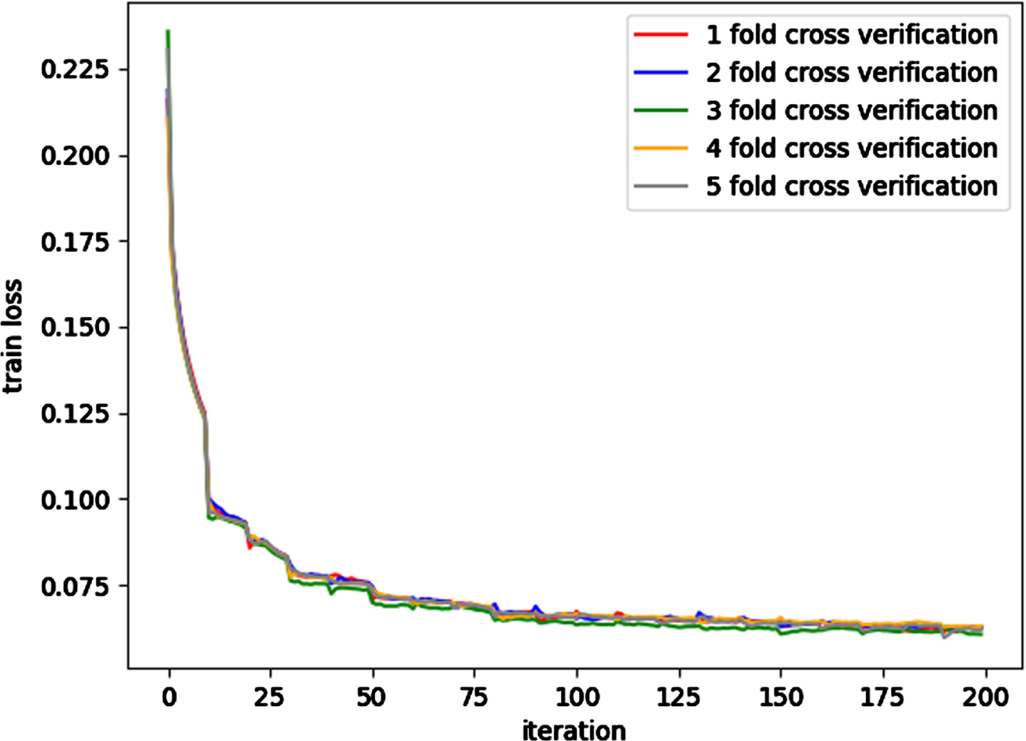
Cross-verify the variation diagram of experimental training loss function values.

5.5 Ablation experiment

In Section 4, we proposed the integration of pedestrian position, size information, pedestrian head direction, and vehicle self-motion information as crucial components of our trajectory prediction model, and subsequently proposed our predictive network. To validate the efficacy of these modules in processing the aforementioned information, This study featured a series of ablation experiments on the MOT16 pedestrian dataset and Daimler dataset, testing the performance of remaining parts when certain network structures within the model were removed, in order to assess whether the model can better utilize this information to achieve more accurate pedestrian trajectory predictions. We compared the following four experimental groups:

Group A: only considered the location and size of pedestrians;

Group B: considered the position, size information of the pedestrians, and the direction of pedestrian’s head;

Group C: considered pedestrian position, size information, and vehicle self-motion information;

Group D: considered pedestrian position, size information, pedestrian head direction, and vehicle self-motion information (our proposed model).

Table 2 presents the results from the ablation experiment:

Table 2
Ablation experiment table

Experiments Features Evaluation

Information Metrics

Tra Head Ego ADE FDE

A ✓ - - 0.43 0.72

B ✓ ✓ - 0.42 0.70

C ✓ - ✓ 0.41 0.69

D(Ours) ✓ ✓ ✓ 0.40 0.68

Experiments	Features	Evaluation
A	✓	-	-	0.43	0.72
B	✓	✓	-	0.42	0.70
C	✓	-	✓	0.41	0.69
D(Ours)	✓	✓	✓	0.40	0.68

Following the design and analysis of these experiments, the performance of Groups B and C exceeded that of Group A, attesting to the effectiveness of adding pedestrian head direction and vehicle self-motion information. Group D exhibited the optimal prediction performance, with significantly lower ADE and FDE compared to the other groups. The ADE index of group D decreased by 7.5% and the FDE index dropped by 5.8% when compared to Group A. These experimental outcomes demonstrate that an improved trajectory prediction model can be achieved by integrating these three strategies.

Following the introduction of our proposed methodology, both ADE and FDE indices exhibited improvements, with ADE metrics showing the most significant enhancement during testing. The ADE index reflects the variance of the prediction error at diverse points during the prediction process. This suggests that the proposal of feature fusion for pedestrian features and vehicle self-motion information, in addition to the feature addition to the interaction module, can efficiently decrease the prediction error at various time points.

5.6 Analysis of model training results

In this subsection, we performed 1000 iterations of network training. After each iteration, we used the validation set to calculate the change in the loss function of the current network on the validation set. The changes of the loss function values on the training and validation sets with respect to the training iterations are depicted in Fig. 11. In the figure, the solid blue line signifies the change in the training set’s loss function, while the solid orange line represents the change in the validation set’s loss function. The horizontal axis represents the training iterations, and the vertical axis represents the loss function value of the corresponding training iteration. The experimental results show that as the number of training iterations increases, the training set loss function decreases from 0.22 to below 0.05, indicating that the model’s training has reached a relatively stable convergence state. During the early training phase, the loss function of the validation set also decreases with an increase in training iterations. However, after roughly 200 iterations, the validation set’s loss function stops declining, demonstrating that the model has reached convergence. Hence, to ensure the model’s generalization capability, training should be ceased once the iterations reach 200, and the model parameters at this point should be used as the final parameters.

Fig. 11

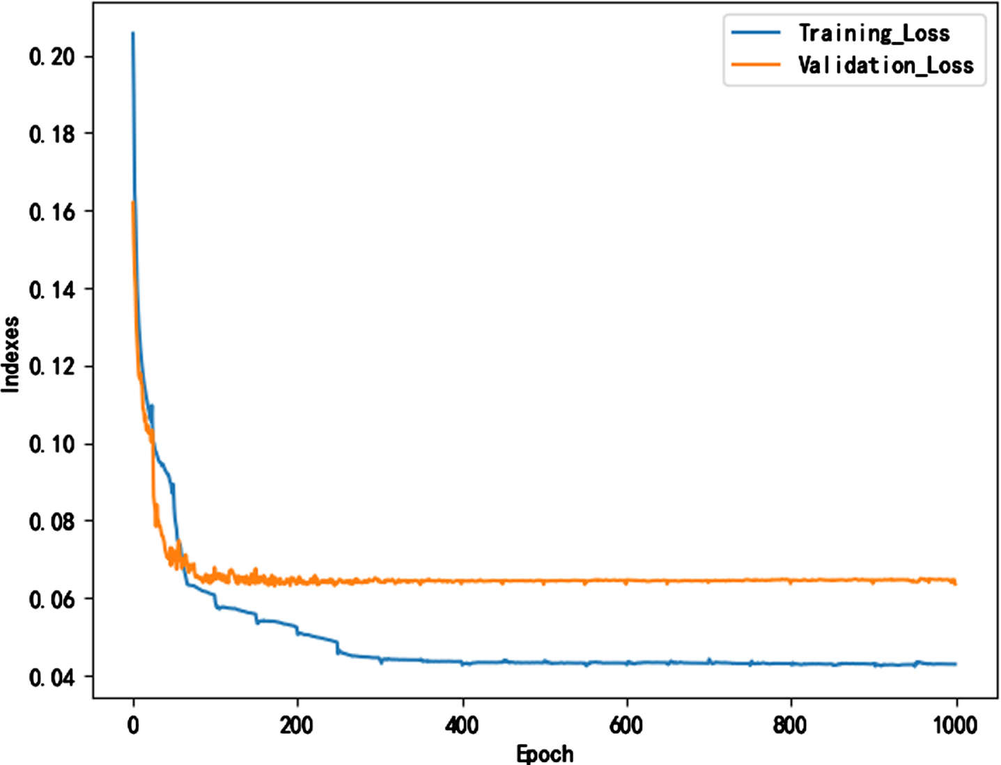
The changing process of model training loss function value.

6 Analysis and discussion of experiment results

6.1 Comparative analysis of experiment results

To fairly evaluate the accuracy of trajectory prediction between the proposed algorithm and other algorithms, we have selected eight different deep learning-based pedestrian trajectory prediction algorithms for comparison. The performance of our proposed model was measured using ADE and FDE indices, as presented in Table 3. To ensure the fairness of the comparative experiments, all models were fed with video inputs of the same duration and tasked to predict pedestrian trajectories over an identical time span (input video length of 3.2 seconds, forecasting pedestrian trajectory for the subsequent 3.2 seconds), guaranteeing that different algorithms are evaluated under equivalent conditions. In terms of learning parameter selection, we referred to the recommended settings in the original papers for each model and, from that baseline, we fine-tuned the parameters. Multiple adjustments were carried out to identify the optimum model parameters.

Table 3
Experimental results comparison of several methods to our proposed model SGPN are shown

Model ADE FDE

Daimler Mot16 Average Daimler Mot16 Average

LSTM 0.92 0.72 0.82 2.05 1.29 1.67

S-LSTM 0.73 0.54 0.63 1.49 1.03 1.26

S-GAN [30] 0.82 0.65 0.74 1.63 1.09 1.36

Sophie [34] 0.68 0.47 0.58 1.39 0.90 1.14

SR-LSTM [21] 0.65 0.42 0.54 1.28 0.83 1.06

Next [31] 0.59 0.40 0.49 1.17 0.80 0.99

STGAT [32] 0.61 0.38 0.49 1.15 0.78 0.96

FPL [33] 0.56 0.30 0.43 0.90 0.61 0.76

SGPN (Ours) 0.48 0.32 0.40 0.83 0.53 0.68

Model	ADE	FDE
LSTM	0.92	0.72	0.82	2.05	1.29	1.67
S-LSTM	0.73	0.54	0.63	1.49	1.03	1.26
S-GAN [30]	0.82	0.65	0.74	1.63	1.09	1.36
Sophie [34]	0.68	0.47	0.58	1.39	0.90	1.14
SR-LSTM [21]	0.65	0.42	0.54	1.28	0.83	1.06
Next [31]	0.59	0.40	0.49	1.17	0.80	0.99
STGAT [32]	0.61	0.38	0.49	1.15	0.78	0.96
FPL [33]	0.56	0.30	0.43	0.90	0.61	0.76
SGPN (Ours)	0.48	0.32	0.40	0.83	0.53	0.68

As can be seen from Table 3, our methodology significantly outperforms other trajectory prediction methods. The predictive performance of all algorithms is notably superior to that of traditional LSTM algorithms. S-LSTM, through social pooling, utilizes the LSTM states between adjacent pedestrians, lowering ADE and FDE slightly, but it doesn’t consider the characteristic information of pedestrians themselves in the scene, resulting in a lack of pedestrian intent expression. If the effect of self-motion on the position of people in the frame is not explicitly considered, temporal models like S-LSTM and S-GAN will fail to learn meaningful temporal dynamics, resulting in their predictions being highly unstable. SR-LSTM, which incorporates global context information, predicts group movement trajectories better. ADE and FDE are modestly lowered, but it likewise neglects the feature information of individual pedestrians and is insufficient in capturing crucial movements, lacking an expression of pedestrian intent. FPL has the best prediction result among these eight algorithms, it fully utilizes pedestrian feature information but overlooks interaction between pedestrians, ADE and FDE for the predicted model are 0.43 and 0.76 respectively. Our method takes into consideration the features of pedestrians themselves. We introduce a double attention mechanism into our model and include pedestrian feature information and vehicle self-movement information into the trajectory prediction module. The proposed SGPN outperforms all other models, with FDE at 0.68, significantly lower than the second-best model FPL, and FDE error decreased by about 10.5%.

The task of pedestrian trajectory prediction necessitates real-time applicability in autonomous driving systems, thus, a real-time performance evaluation of proposed algorithms is essential. This article comparatively investigates the operation speeds of several deep learning network-based models. The real-time performance evaluation was conducted on a platform with Inter Xeon E5-2620 v4 CPU and NVIDIA GeForce RTX 2080Ti GPU, as indicated in Table 4.

Table 4

Comparison of inference speeds of different trajectory prediction models

Model	Forecast time (ms)	Multiple relation
S-LSTM	2.64	1 ×
S-GAN	2.28	1.16 ×
STGAT	0.33	8 ×
FPL	0.21	12.57 ×
SGPN (Ours)	0.09	29.33 ×

The results reveal that the proposed algorithm functions rapidly, thus implying superior real-time performance. Specifically, the SGPN model can generate pedestrian trajectories in merely 0.089 milliseconds, which is 29.33 times and 25.33 times faster than the S-LSTM model and S-GAN model, respectively. Although the FPL model solely employs a CNN network, its operation speed decreases due to the use of a skeleton extraction algorithm during feature extraction. Compared to the relatively high-speed operation of FPL, SGPN operates at 2.33 times the speed.

6.2 Visualization of experimental results

This section primarily qualifies the predictive performance of the model, demonstrating the visualization results of pedestrian trajectory predictions for the Daimler dataset and MOT16 pedestrian dataset, as shown in Fig. 12 and Fig. 13. In this study, we utilized YOLOv7 in conjunction with deepsort for pedestrian detection and tracking. We have distinguished between single and multiple pedestrian scenes based on different pedestrian densities.

Fig. 12

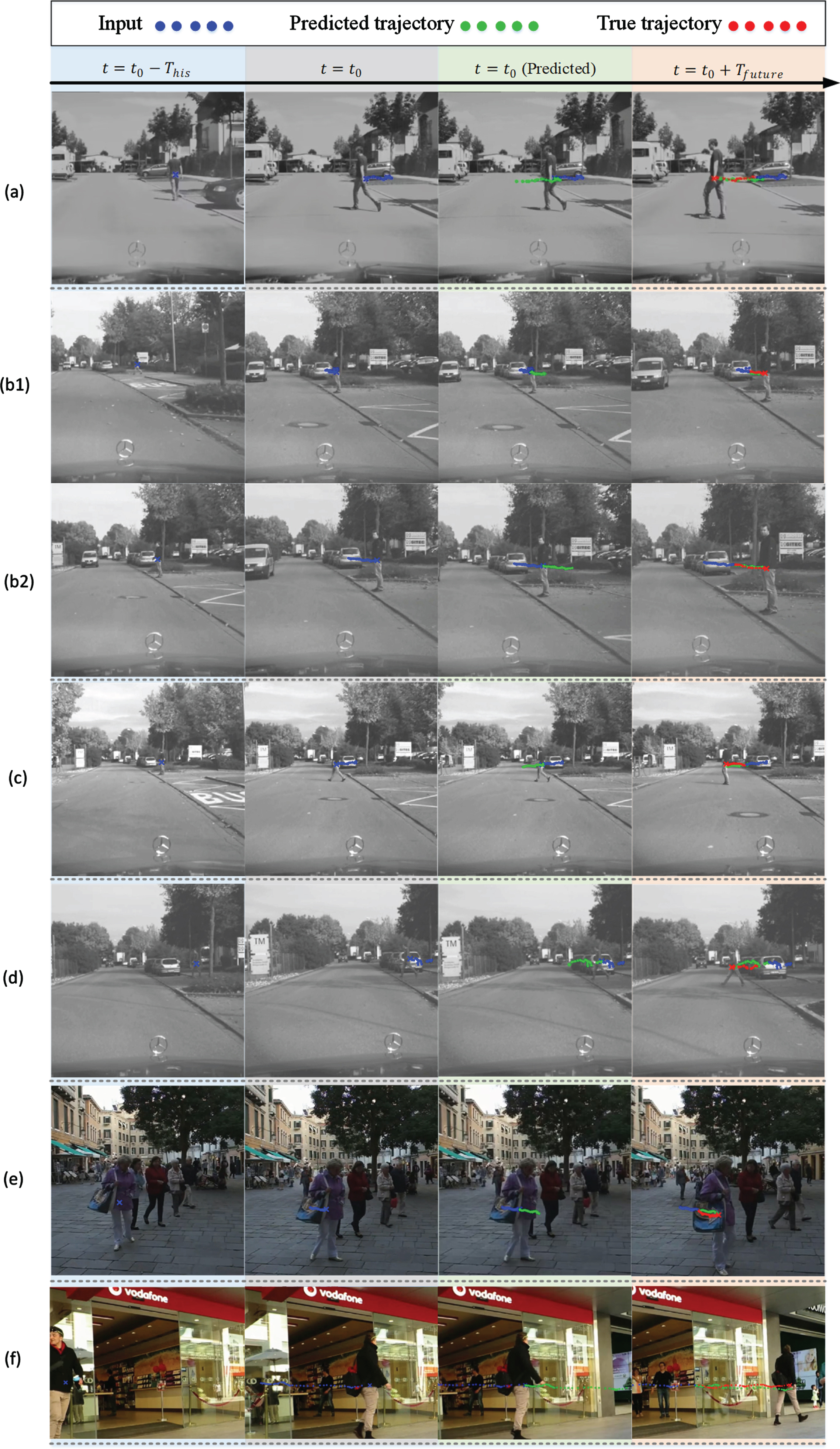
Examples of single pedestrian trajectory predictions of video. Figure 12(a) to Fig. 12(d) demonstrate trajectory predictions for four different types of pedestrian movement on the Daimler dataset, namely Bending In, Stopping, Crossing, and Starting; Figure 12(e) and Fig. 12(f) show the trajectory predictions for specified pedestrians from part of the MOT16 pedestrian dataset.

Fig. 13

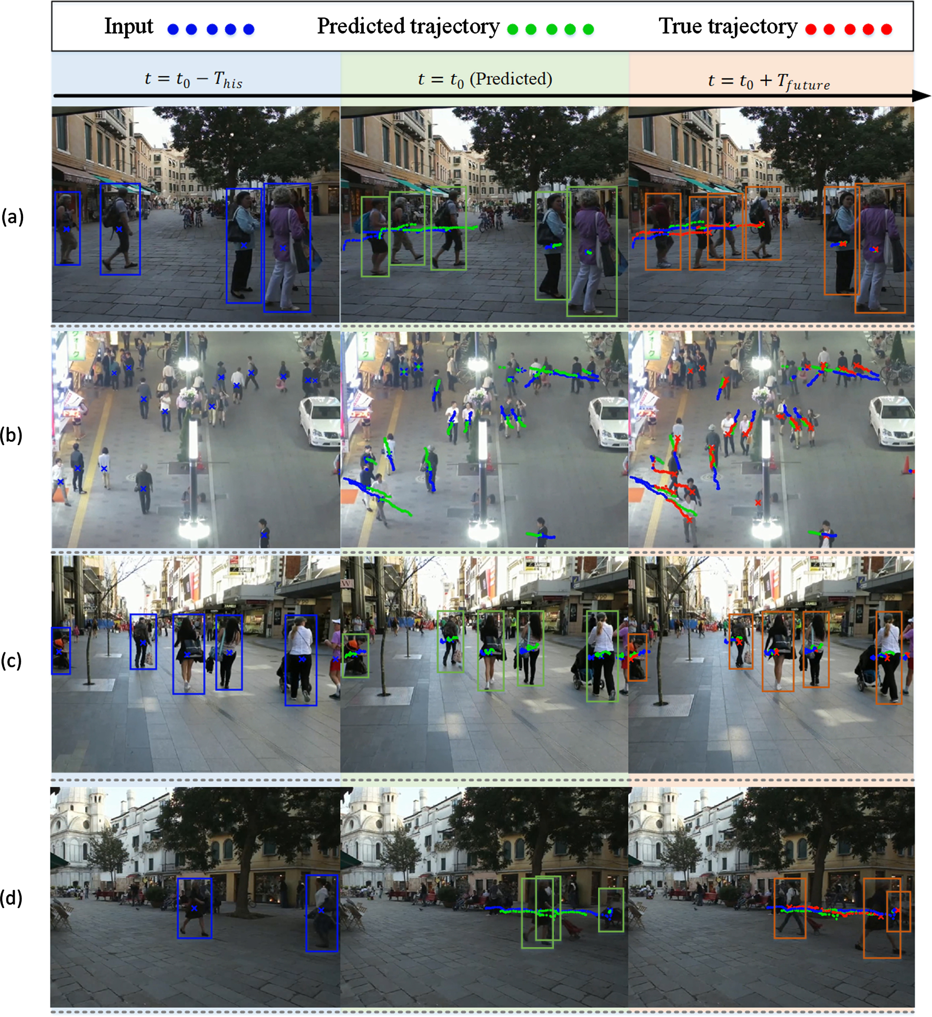
Examples of trajectory predictions for multiple pedestrians in video. Figure 13(a) to Fig. 13(d) illustrate the trajectory predictions for groups of pedestrians or specific multiple pedestrians in the MOT16 pedestrian dataset.

Each row represents the visualization of pedestrian trajectory sequences within a sequence of video frames. Figure 12 includes four image frames, and Fig. 13 includes three. For each frame, the left indicates the frame at time t - 10, and the right indicates the frame at time t + 10. Each image displays the historical trajectory sequence, actual future trajectory sequence, and predicted future trajectory sequence of the target pedestrian. For Fig. 12, we give both the position of the pedestrian at time t₀ and the predicted future trajectory sequence at this time. For Fig. 13, the middle image demonstrates the predicted future trajectory sequence at time t₀. In these diagrams, blue lines depict the pedestrian’s historical trajectory sequence, green lines represent the actual future trajectory sequence, and red lines illustrate the predicted future trajectory sequence.

6.3 Discussion

In studies related to pedestrian trajectory prediction, traditional prediction methods based on shallow learning have achieved satisfactory prediction results in handling simple or standardized problems. However, when faced with real-life complex traffic scenarios, the prediction accuracy would be limited and the generalization capability of the shallow learning model is relatively weak. Most trajectory prediction methods based on deep learning overly simplify the pedestrian and environment feature information; some models lack a description of crucial movement information. For instance, S-LSTM and G-LSTM methods overly rely on location information and cannot adequately express the actual conditions in complex traffic scenarios.

In contrast to a single prediction network, our research breaks away from prior studies on pedestrian trajectory prediction, proposing a newly developed deep learning-based SGPN model. Firstly, this model combines the feature extraction capability of CNN and the superior handling of sequence data by LSTM, thereby adapting better to the trajectory prediction task. The design of LSTM network has been revised, and LSTM was optimized twice to resolve the feature expression issue of an individual pedestrian in the time domain and a group of pedestrians in the space domain respectively. Secondly, we introduced a dual attention mechanism for the model to itself and the scene, aiding the model in adaptive feature selection and weighting allocation of the information in history. The dual attention mechanism avoids insufficient scenario descriptions and inadequate descriptions of pedestrian states potentially caused by a singular attention mechanism.

Four structural parts of SGPN have undergone deep optimization and are provided with specific mathematical formulas. These improvements will help enhance the accuracy of prediction. Our model possesses high accuracy when predicting pedestrian trajectories and has been supported through numerous experimental investigations. Section 6.1 and 6.2 provide a quantitative and qualitative analysis of the model respectively, enabling a precise evaluation of the strengths and weaknesses of the model. The prediction accuracy errors ADE and FDE of our model are 0.40 and 0.68 respectively, significantly superior to other algorithmic models. This paper surpasses traditionally oversimplified prediction models, accurately depicting pedestrian movement patterns in real-life scenarios.

Understanding and modeling the uncertainty in individual behaviors is crucial for enhancing the accuracy of pedestrian trajectory predictions. Although our SGPN model, with its dedicated modules, learns the interactions between pedestrians and their environment from historical data, thus effectively handling some uncertain factors and predicting trajectories in complex scenarios, there is still room for improvement in learning efficacy under data scarcity conditions. Tutsoy et al. [35] introduced an improved genetic algorithm coupled with fractional-order polynomial models for long-term multidimensional prediction, which has been particularly successful in addressing uncertainties in sparse data scenarios, and they have provided a stable polynomial parameter update mechanism to accommodate annual data refreshes. Their methodology offers insights into potential strategies for augmenting the adaptability of our model in uncertain contexts. For future work, we will consider incorporating a similar mathematical framework or algorithm within the FFM of our SGPN model to further enhance predictive accuracy under uncertainty.

7 Conclusion

In the context of autonomous driving, accurate prediction of pedestrian trajectories is crucial for mitigating road safety risks. While existing deep learning models have made advancements in many aspects, they typically fall short in adequately addressing pedestrian interactions in complex environments. Our proposed SGPN model employs an innovative LSTM cell structure optimization and an advanced dual-attention mechanism, substantially improving the accuracy of pedestrian trajectory predictions.

To enhance the comprehensive value of our study, a comparative analysis with other scholarly works was conducted. In the realm of pedestrian trajectory forecasting, deep learning-based methods such as S-GAN, S-LSTM, and FPL predominate. However, these models reveal constraints when addressing complex pedestrian interactions within intricate scenarios. Specifically, the existing models warrant enhancement in the domain of capturing pedestrian characteristic features and key interactive dynamics. In contrast, our research bolsters the learning capabilities of pedestrian features and delves deeper into pivotal interactions between pedestrians and environment. Utilizing datasets like the MOT16 pedestrian dataset and the Daimler pedestrian benchmark dataset, our SGPN yielded an average FDE of 0.68, which represents a notable improvement in performance over other models, with the next best model FPL achieving an average FDE of 0.76. These outcomes distinctly manifest the superior proficiency of SGPN in interpreting complex individual behavioral dynamics, as well as making a significant contribution to modeling spatial interactions, which includes both inter-pedestrian interaction and the pedestrian-environment interplay.

The model and methods proposed in our study have various potential extensions and applications for future research. Considering the integration of spatial and temporal information, our work holds significance for related research, providing theoretical support and practical insights. In future work, we plan to incorporate richer scene information and consider integrating the latest advancements in deep learning to enhance feature extraction effectiveness, thereby further improving the predictive performance and generalizability of our model.

Footnotes

Acknowledgments

Research supported in part by grant for the Key Research and Development Program of Shaanxi Province of China (2019GY-097, 2021GY-131), Yulin Science and Technology Plan Project (CXY-2020-037), Xi’an Science and Technology Plan Project (2020KJRC0068), and Innovation Capability Support Program of Shaanxi (2020TD-021).

References

Golchoubian

, Ghafurian

, Dautenhahn

et al., Pedestrian trajectory prediction in pedestrian-vehicle mixed environments: A Systematic Review[J], IEEE Transactions on Intelligent Transportation Systems, 2023. doi: 10.1109/TITS.2023.3291196.

Poliak

, Beu

and Lazaroiu

, Violations of social regulation and traffic accidents in road freight transport[J], Archiwum Motoryzacji 97(3) 2022. https://doi.org/10.14669/AM/155050.

Shi

, Ye

, Shiwakoti

et al., A review of experimental studies on complex pedestrian movement behaviors[J], CICTP 2015 (2015), 1081–1096.

, Eiffert

, Shan

et al., Attentional-GCNN: Adaptive pedestrian trajectory prediction towards generic autonomous vehicle use cases[C], 2021 IEEE International Conference on Robotics and Automation (ICRA), IEEE (2021), 14241–14247.

Novak

et al., Big Data-driven Governance of Smart Sustainable Intelligent Transportation Systems: Autonomous Driving Behaviors, Predictive Modeling Techniques, and Sensing and Computing Technologies, Contemporary Readings in Law and Social Justice (2022), 100–117. doi: 10.22381/CRLSJ14220226.

Hema

D. Deva

and Kumar

K. Ashok

, Novel algorithm for multivariate time series crash risk prediction using CNN-ATT-LSTM model[J], Journal of Intelligent & Fuzzy Systems 43(4) (2022), 4201–4213.

Tai

K.S.

, Socher

and Manning

C.D.

, Improved semantic representations from tree-structured long short-term memory networks[J], arxiv preprint arxiv:1503.00075, 2015.

Coué

, Pradalier

, Laugier

et al., Bayesian occupancy filtering for multitarget tracking: an automotive application[J], The International Journal of Robotics Research 25(1) (2006), 19–30.

Helbing

and Molnar

, Social force model for pedestrian dynamics[J], Physical review E 51(5) (1995), 4282.

10.

Schneider

and Gavrila

D.M.

, Pedestrian path prediction with recursive bayesian filters: A comparative study[C], German Conference on Pattern Recognition. Berlin, Heidelberg: Springer Berlin Heidelberg (2013), 174–183.

11.

Pavlovic

, Rehg

J.M.

and MacCormick

, Learning switching linear models of human motion[J], Advances in Neural Information Processing Systems (2000), 13.

12.

Bhaskara

, Viswanath

and Bera

, Trajectory Prediction for Robot Navigation using Flow-Guided Markov Neural Operator[J], arXiv preprint arXiv:2309.09137, 2023.

13.

Shaojie

, Kun

, Nan

et al., A trajectory prediction algorithm based on Gaussian mixture model [J], Journal of Software 26(05) (2015), 1048–1063.

14.

Rhinehart

and Kitani

K.M.

, First-person activity forecasting from video with online inverse reinforcement learning[J], IEEE Transactions on Pattern Analysis and Machine Intelligence 42(2) (2018), 304–317.

15.

Park

H.S.

, Hwang

J.J.

, Niu

et al., Egocentric future localization[C], Proceedings of the IEEE Conference on Computer Vision and Pattern Recognition (2016), 4697–4705.

16.

Xie

, Shu

, Todorovic

et al., Learning and inferring dark matter and predicting human intents and trajectories in videos[J], IEEE Transactions on Pattern Analysis and Machine Intelligence 40(7) (2017), 1639–1652.

17.

Elman

J.L.

, Finding structure in time[J], Cognitive Science 14(2) (1990), 179–211.

18.

Chung

, Gulcehre

, Cho

K.H.

et al., Empirical evaluation of gated recurrent neural networks on sequence modeling[J], arXivpreprint arXiv:1412.3555, 2014.

19.

Topal

M.E.

and Tutsoy

, Vision-Based Vehicle Detection and Driver Intention Recognition[C], Proceedings of the 4th International Congress on Engineering Sciences and Multidisciplinary Approaches, 2022.

20.

Chaoming

, Prediction and analysis of sphere motion trajectory based on deep learning algorithm optimization[J], Journal of Intelligent & Fuzzy Systems 37(5) (2019), 6275–6285.

21.

Zhang

, Ouyang

, Zhang

et al., Sr-lstm: State refinement for lstm towards pedestrian trajectory prediction[C], Proceedings of the IEEE/CVF Conference on Computer Vision and Pattern Recognition (2019), 12085–12094.

22.

Alahi

, Goel

, Ramanathan

et al., Social lstm: Human trajectory prediction in crowded spaces[C], Proceedings of the IEEE Conference on Computer Vision and Pattern Recognition (2016), 961–971.

23.

Pellegrini

, Ess

, Schindler

et al., You’ll never walk alone: Modeling social behavior for multi-target tracking[C], 2009 IEEE 12th International Conference on Computer Vision, IEEE (2009), 261–268.

24.

Lerner

, Chrysanthou

and Lischinski

, Crowds by example[C], Computer Graphics Forum 26(3) (2007), 655–664.

25.

Rashmi

, Chiu

and Bera

, SGLSTM: Social group LSTM for robot navigation through dense crowds, arXiv preprint arXiv:2303.04320, 2023.

26.

Bisagno

, Zhang

and Conci

, Group lstm: Group trajectory prediction in crowded scenarios[C], Proceedings of the European Conference on Computer Vision (ECCV) Workshops, 2018.

27.

Fernando

, Denman

, Sridharan

et al., Soft+ hardwired attention: An lstm framework for human trajectory prediction and abnormal event detection[J], Neural Networks 108 (2018), 466–478.

28.

Cordts

, Omran

, Ramos

et al., The cityscapes dataset for semantic urban scene understanding[C], Proceedings of the IEEE Conference on Computer Vision and Pattern Recognition (2016), 3213–3223.

29.

Milan

, Leal-Taixé

, Reid

et al., MOT16: A benchmark for multi-object tracking[J], arXiv preprint arXiv:1603.00831, 2016.

30.

Gupta

, Johnson

, Fei-Fei

et al., Social gan: Socially acceptable trajectories with generative adversarial networks[C], Proceedings of the IEEE Conference on Computer Vision and Pattern Recognition (2018), 2255–2264.

31.

Liang

, Jiang

, Niebles

J.C.

et al., Peeking into the future: Predicting future person activities and locations in videos[C], Proceedings of the IEEE/CVF Conference on Computer Vision and Pattern Recognition (2019), 5725–5734.

32.

Huang

, Bi

, Li

et al., Stgat: Modeling spatial-temporal interactions for human trajectory prediction[C], Proceedings of the IEEE/CVF International Conference on Computer Vision (2019), 6272–6281.

33.

Yagi

, Mangalam

, Yonetani

et al., Future person localization in first-person videos[C], Proceedings of the IEEE Conference on Computer Vision and Pattern Recognition (2018), 7593–7602.

34.

Sadeghian

, Kosaraju

, Sadeghian

et al., Sophie: An attentive gan for predicting paths compliant to social and physical constraints[C], Proceedings of the IEEE/CVF Conference on Computer Vision and Pattern Recognition (2019), 1349–1358.

35.

Tutsoy

and Tanrikulu

, A Machine learning-based 10 years ahead prediction of Departing foreign visitors by Reasons: A Case on Türkiye, Applied Sciences, 2022.

Model	ADE			FDE
	Daimler	Mot16	Average	Daimler	Mot16	Average
LSTM	0.92	0.72	0.82	2.05	1.29	1.67
S-LSTM	0.73	0.54	0.63	1.49	1.03	1.26
S-GAN [30]	0.82	0.65	0.74	1.63	1.09	1.36
Sophie [34]	0.68	0.47	0.58	1.39	0.90	1.14
SR-LSTM [21]	0.65	0.42	0.54	1.28	0.83	1.06
Next [31]	0.59	0.40	0.49	1.17	0.80	0.99
STGAT [32]	0.61	0.38	0.49	1.15	0.78	0.96
FPL [33]	0.56	0.30	0.43	0.90	0.61	0.76
SGPN (Ours)	0.48	0.32	0.40	0.83	0.53	0.68