Performance evaluation of Twitter datasets on SQL and NoSQL DBMS

Abstract

Twitter has grown significantly in the past several years and provides a new vector for data collection, offering individual users and companies valuable insights. This presents a technical challenge to collect and analyze all the data in an efficient manner. Traditional relational databases have not been able to provide acceptable response times that this new problem presents, and focus has started shifting to newer technologies such as NoSQL databases. In this paper, we try to answer a question as follows: “If I want to store and access millions of tweets for data analysis, which database systems should I choose?” We selected four popular SQL and NoSQL database systems and tested on different twitter dataset varying from one million to fifty million tweets. Each workload test involves running a core set of data operation commands. The experiment results are promising and provide guideline for choosing the most efficient database systems based on different user requirements.

Keywords

SQL NoSQL JSON big data Twitter

1. Introduction

Created in 2006, Twitter is a microblogging, social networking service designed around messages limited to 140-characters called “tweets”. As this platform is user-driven with few rules (aside from local or federal laws that already exist), users are free to tweet anything they want, from mundane descriptions or pictures of their meal, to complaining about a company’s bad customer service, or even to have a written protest of policies enacted by a government. The service is free to use, and has been important in fast dissemination of information from news-worthy events (such as the Egyptian government protest and overthrow) to other events such as the devastation felt by millions of fans when a member left the musical group One Direction. In fact, popular web comic XKCD made a point that with the low threshold of tweet content and the speed of electricity, people outside of the radius of an earthquake may receive information about the quake via Twitter before they can even feel the seismic waves themselves [13].

This means that if anyone can tweet about anything they want, there are a lot of tweets that must exist, constantly being created, stored, and viewed. This also means that tweets amount to a significant chunk of data that may be studied for non-profit reasons like research, and for-profit reasons like advertising and polling a company’s user base. Handling hundreds of millions of tweets daily [9] and the availability of a public API to download and stream new tweets has allowed any person and company to freely find and discover trends on opinions and events in real-time.

A technical challenge comes into play when needing to store and access millions of pieces of data constantly. Traditional SQL-based relational database systems have slowly started adapting to the newly unique needs. The data response from the Twitter API is in the form of JavaScript Object Notation (JSON). The question as follows: “If I want to store and access millions of tweets for myself, which Database Management Systems (DBMS) should I choose?” With different amounts of native support for the JSON format, it raises the question of how comparable in performance they are for storing tweets. Additionally, the sheer number of tweets being created makes having an ideal dataset to be millions of tweets in size, at a minimum.

In this paper, we test and compare the performance of four popular DBMS: Microsoft SQL Server, PostgreSQL, MongoDB and Redis. Each DBMS has different levels of support for JSON: SQL Server has no native JSON support, and PostgreSQL only gained support in late 2013. NoSQL-based systems such as MongoDB launched in 2009 with native support in a derivative format called Binary JSON (BSON), and Redis allows storage of JSON but does not specifically support that data type natively. We explore and present our findings using datasets consist of millions of tweets, tested on and compare the performance between these four DBMS. Our experimental results show some interesting findings and provide guidelines on how to choose the most efficient DBMS based on different user needs.

2. Background and related work

2.1. Tweets and big data, collecting and storing

Twitter has grown significantly in the past several years and provides a new vector for data collection, offering companies valuable insight in its users and customers. This presents a technical challenge to collect and analyze all the data in an efficient manner. “Big Data”, a term used to describe the massive influx of data being handled and studied (not exclusive to tweets), has been a large driving force for NoSQL adoption [16]. Traditional relational databases have not been able to provide acceptable response times that this new problem presents, and focus has started shifting to newer technologies such as NoSQL-based DBMS.

Big Data can be described in three V’s: volume, variety and velocity. The sheer volume of data is difficult for SQL-based solutions because scalability was not one of the primary concerns decades ago. Though certainly scalable, database servers of the past were run on highly specialized hardware, needing more of the same or similar hardware to expand and scale out. NoSQL emphasizes horizontal scaling on commodity hardware, allowing a much lower cost to scaling out. Consistency, as a part of atomicity, consistency, isolation, durability (ACID), takes a back seat in NoSQL by not guaranteeing it. Instead, redundant data is kept with “eventual consistency”, which states that if no new updates are made to a given data item, eventually all accesses to that item will return the last updated value. Redundant data also allows for lower read latency as there would be a higher chance of “finding” the data.

In SQL-based DBMS, the schema is set and defined in advance, and additional data added to the set must adhere to the schema. For guarantees and a system of checks on data, such as type, a strict schema can be helpful. NoSQL eschews this strict need and is flexible with its schema by not explicitly requiring conformity. This gives the developer/DBA more power (and responsibility) in maintaining the database by grouping together similar data without it all needing to be exactly the same. In some types of databases, such as key-value stores, the database itself knows nothing about the data it is storing.

New data is constantly added and stored, with low read latency still strongly desired. ACID overhead for all the data is high, and some users don’t need all its data all the time, allowing consistency guarantees to be dropped in favor for faster performance. NoSQL does not always have ACID guarantees (it may be implemented by the developer at the application level), and better scalability helps maintain low read latency alongside redundant data.

NoSQL is currently the hot new solution to aid companies and developers in handling the challenges that Big Data brings.

2.2. DBMS types

Relational database systems based on SQL-syntax have existed since the 1970s in many forms, and have been widely used as the primary means to host databases. Strong support for ACID and transactions make them extremely dependable and resilient. In areas in which traceability and dependability are paramount (e.g. banking and finance), the framework of ACID will not be replaced by something else. The overhead of ACID makes SQL-based DBMS slower than alternatives that do not strictly conform to it.

Despite the abbreviation of the term NoSQL suggests its meaning “No SQL” or “non SQL”, many software vendors prefer it to be viewed as “Not Only SQL”, representing alternative methods for databases to store data [2].

The methods used by NoSQL-based DBMS are not new, and are also as old as SQL-based ideas. However, NoSQL products most popular today have been heavily influenced by Google BigTable, an in-house data storage system first introduced in [7,12].

Different methods of storing data include:

column-store – columns consist of a unique name, value (content), and timestamp;

document-oriented store – store objects as documents (frequently JSON);

key-value store – use an associative array with a collection of key, value pairs;

graph store – based on graph structure.

NoSQL does not guarantee ACID like SQL-based systems, and is in fact sometimes classified as BASE – Basically Available, Soft state, Eventual Consistency. Application developers do have more leeway in the details of storage and implementation, at the risk of greater dependence on the developer. For the two NoSQL DBMS used in our experiment, MongoDB is a document-oriented store, and Redis is a key-value store stored in-memory.

2.3. DBMS tested

Microsoft SQL Server 2014 is continuation of their long-running DBMS products, with version 1.0 originally released in 1989. SQL Server is a relational DBMS and offers multiple tiers of its product, ranging from the free Express to the not-free Enterprise editions. The editions differ in features available, such as high availability, security, and replication options, and database size and hardware support (e.g. limitation on number of processors and cores usable). The edition used for testing is the Enterprise edition, whose limitations are bound by hardware and not software. The many extra features such as the previously mentioned high availability and replication are not used. The version used is 12.0.4100.1. The Python library used is pymssql 2.1.1.

PostgreSQL is a relational DBMS developed officially by the PostgreSQL Global Development Group, consisting of different companies and individuals [15]. The software is free and open source software and released under the PostgreSQL License. The version used is 9.4.1 64-bit. The Python library used is psycopg 2 2.6.1.

MongoDB is a document-oriented database with dynamic schemas originally released in its current form as a standalone database product in 2009, released under the GNU Affero General Public License and is free and open source software. As of this writing, it is the most popular database of its type [6]. The version used is 3.0.1. The Python library used is pymongo 3.0.3.

Redis is an in-memory data structure server, supporting several different types of data structures such as lists, sets, hashes and bit arrays. The entire dataset is hosted in physical memory, with changes saved to disk in user-specified intervals. The version used is 2.8 using the Windows port, despite Redis’s only officially supported platform being on Linux. This decision was made to keep its environment similar to other DBMS already running on Windows. The Python library used is redis 2.10.3.

2.4. Related work

There are several papers in literature provide comparison between NoSQL databases and relational DBMS in terms of types of NoSQL data store, query languages used in NoSQL, advantages and disadvantages of NoSQL over relational DBMS [2,4,8,14]. However, there are very few papers that have dealt specifically with benchmarking and comparing SQL and NoSQL DBMS. One such is [10] which only used datasets sized from 148 to 12,416 tuples/documents, and only compared MongoDB to SQL Server. Paper [1] benchmarked only the NoSQL DBMS MongoDB, ElasticSearch, OrientDB, and Redis between each other with dataset sizes ranging from 1,000 to 100,000 records.

There are more informal sources for comparisons, specifically on personal and company blogs. An older but apparently well-known benchmark is the Yahoo! Cloud Serving Benchmark (YCSB) [5], an open source tool initially written in 2010 to test many different types of DBMS, including SQL and NoSQL DBMS. Some of the workloads defined by that benchmark have also been adopted for testing in this paper. The scope of our work differs from YCSB in that it emphasizes scalability on multiple nodes and processes, and requires elasticity and high availability. Our testing is purposely confined to a single node with no such extra capabilities, rendering YCSB unsuitable for our specific needs.

The computer software company Datastax, which offers an enterprise distribution of the NoSQL DBMS Cassandra, performed an evaluation between three NoSQL DBMS: Cassandra, HBase and MongoDB [3]. Their testing utilized YCSB and revealed Cassandra to outperform the other DMBS products, which is also the product that the company offers as its primary business. Though we don’t necessarily believe their results to be misleading, we withhold some skepticism for a less biased outlook.

Table 1
Core commands

Command SQL Server & PostgreSQL MongoDB Redis

READ SELECT find_one HMGET

UPDATE UPDATE update_one HSET

INSERT INSERT insert_one HMSET

TRUNCATE TRUNCATE db.collection.drop FLUSHDB

Command	SQL Server & PostgreSQL	MongoDB	Redis
READ	SELECT	find_one	HMGET
UPDATE	UPDATE	update_one	HSET
INSERT	INSERT	insert_one	HMSET
TRUNCATE	TRUNCATE	db.collection.drop	FLUSHDB

Table 2

Database schema

DBMS	tweet_id	created_at	user_id	user_name	text
SQL Server	bigint (primary key)	Datetime	bigint	text	text
PostgreSQL	bigint (primary key)	timestamp without timezone	bigint	text	text
MongoDB	None specified, inserted as JSON
Redis	Key set via hashes	Value set via hashes

3. Objectives

In addressing aforementioned challenges when storing and accessing big data, traditional DBMS has difficulty meeting performance requirements. In this paper, we propose to evaluate the performance of four popular DBMS: Microsoft SQL Server, PostgreSQL, MongoDB and Redis. In particular, we test on different twitter dataset varying from one million to fifty million tweets. Our performance evaluation is aimed to fit in the gap between NoSQL-only testing with small dataset sizes, and extremely large scalable cloud systems. Specifically, we look at comparisons between SQL and NoSQL with large dataset sizes without scalability and elasticity requirements.

4. Evaluation methodology

4.1. Workload overview

Each workload test (detailed below) involves running a core set of commands as shown in Table 1 500 times, which is then looped and timed 100 times. Thus, the raw data will show 100 points of data. The dataset involved consists of 50 million tweets with unique tweet IDs (i.e., the “primary” dataset), with tests that use a smaller set of data being a portion of the primary dataset.

For each command requiring something to find (e.g. READ and UPDATE), it uses a list of 500 tweet IDs of existing tweets are randomly chosen. This single list of random tweet IDs is the same for each workload test for the given size. For example, the tests using the 1 million tweet dataset will have a list of 500 tweet IDs spanning its range, and the tests using the 5 million tweet dataset will use a different list that spans the larger range of tweets.

The INSERT command uses a separate, smaller dataset (i.e., the “secondary” dataset) for its tests. The number of tweets is much smaller since the workload requiring doesn’t need much, though the JSON fields remain the same.

4.2. Workload descriptions

Workload A (50/50 R/W) uses UPDATE commands exclusively, searches for 500 tweets using the tweet_id, and updates the user_name field with the string “aaabbb”. Workload B (95/5 R/W) uses 450 READ commands searching for the tweet_id, and 50 UPDATE commands, updating the user_name field with the string “bbbbbb”. Workload C (100 R) uses 500 READ commands, searching using the tweet_id field. Workload Write (100 W) uses 1000 INSERT commands from the secondary dataset, inserted into a new (empty) table and dropped (TRUNCATE or equivalent) at the end of each loop. This is done to keep each insertion “fresh”.

4.3. Schema setup

Table 2 shows database schema across all four DBMS. MongoDB specifically had index created on the tweet_id field, and it appears to be proper setup to create indices for fields that are intended to be searched. Due to hardware constraints, the 25-million and 50-million datasets were unable to be tested in Redis.

Fig. 1.

Data preprocessing steps.

4.4. Test platform specifications

The operating system was installed on Samsung 850 PRO, and all virtual machines (VMs) were hosted only on the Samsung 840 EVO. VMs were managed through the included Hyper-V Manager. VM checkpoints were not utilized to save on disk space.

Each DBMS product was tested in its own VM with its own reserved resources. During testing, only the DBMS being tested had its VM powered on – the others were powered off. Due to disk space constraints on the SSD, hard disk files of VMs had to be moved back and forth between the OS SSD and VM SSD. The details are shown in Tables 3 and 4.

5. Data preprocessing

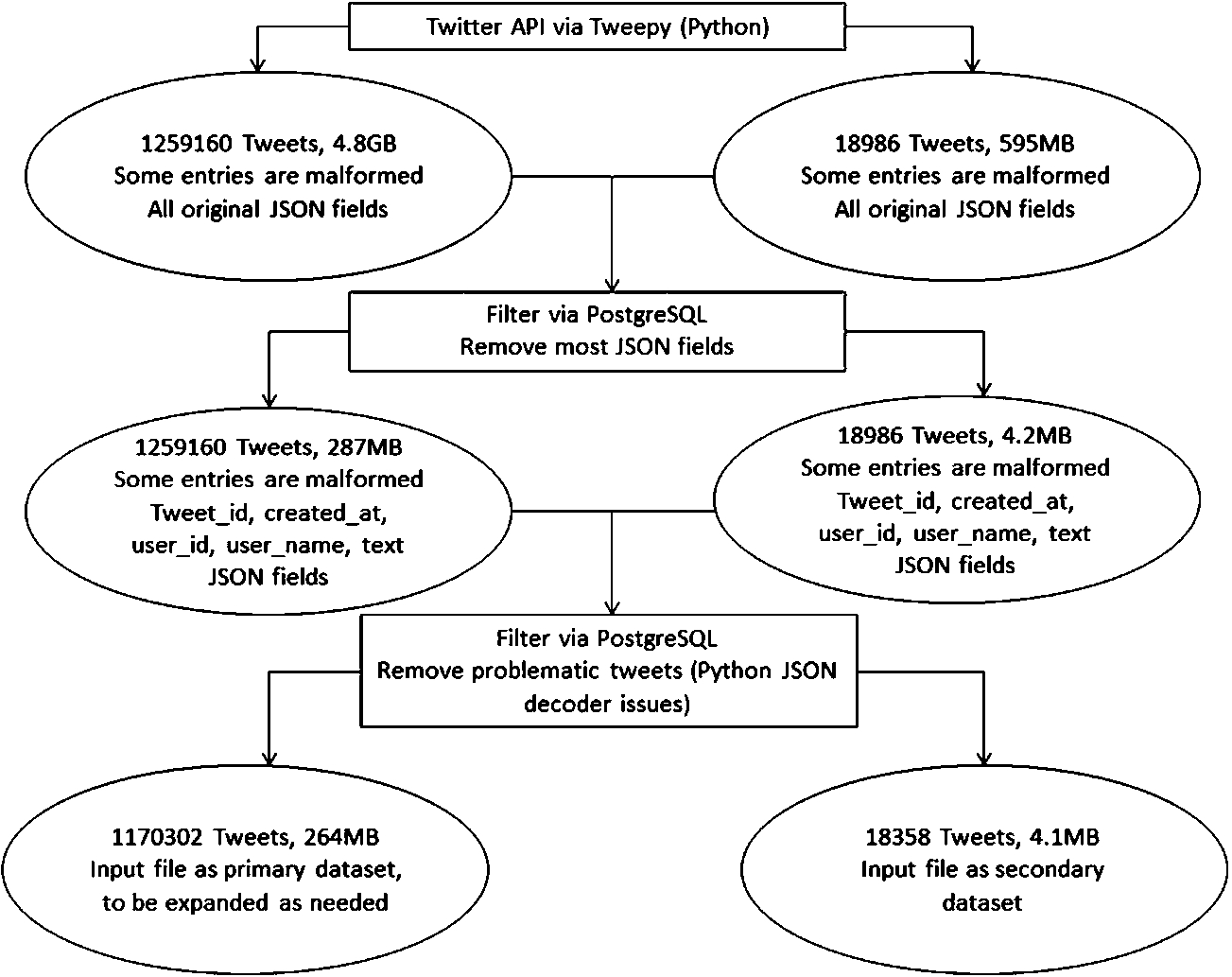
Figure 1 describes how the data was collected, and what was prepared to make it the datasets used in testing.

Table 3
Virtual machine host

Operating System Windows Server 2012 R2 Datacenter

CPU Intel i7-4790 @ 3.60 GHz

Memory 32GB DDR3-1600

SSD Samsung 850 PRO 256 GB (OS)

Samsung 840 EVO 250 GB (VMs)

5.1. Gathering data

The dataset was gathered using Python through Twitter’s Streaming API and each collected tweet was written to a single text file. The filter for tweets contained only common words such as “a”, “the” and “people”, resulting in a quick collection of data. Tweepy, the API library used, does not run without a filter. The resulting dataset contained roughly 1.2 million unique tweets at a disk size of 4.8 GB. There is also a second much-smaller dataset with 18,994 unique tweets at a disk size of 82 MB that is used in Workload Write.

Table 4
Virtual machine setup

Operating System Windows 7 Professional SP1 x64

Disk Size 90 GB

Memory 16384 MB

Virtual Processors 4

Virtual machine reserve (resource control) 100

5.2. Filtering data

The dataset was then imported with a filter into PostgreSQL using its built-in JSON support. During import, only the tweet_id, created_at, user_id, user_ name and tweet text fields were stored. These fields were chosen because they were guaranteed to be populated and to keep the resulting dataset smaller and more manageable.

After the import into PostgreSQL, the data was then exported out as JSON, which now contains only the above five JSON fields. This dataset measured at only 287 MB, with the same number of tweets as the original dataset.

There was an issue with Python’s JSON decoder on some of the tweets regarding delimiters. Due to this issue, the dataset was filtered again through PostgreSQL to remove the offending records. The dataset was then trimmed to 1,170,302 tweets.

The 287 MB-sized primary dataset is now the input file for the next step of processing. The secondary dataset is trimmed to 4.2 MB.

5.3. Expanding the data

Using the 1,170,302 tweets as the base, the data was then duplicated to 50 million records by inserting its own data into itself with an arithmetic increase in tweet IDs (i.e. add a number when inserting again), the commands are shown in Fig. 2.

Fig. 2.

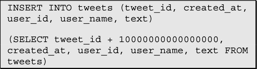
Duplicating tweets commands.

The number added is increased for every subsequent insertion. This allows every record to have a unique tweet ID despite not all the tweets being wholly unique. The datasets with sizes less than 50 million are simply subsets of that data (e.g. 25 million record dataset is exactly half of the 50 million record dataset). The file size of the 50 million record dataset ended up being 11.4 GB.

5.4. Importing data

Each DBMS used the same dataset for its input file, using nearly identical Python scripts, differing only in its connection strings and insert commands. Depending on the DBMS, either only the 50 million record dataset was imported from a text file, or the other datasets were imported from each dataset’s text file. In SQL Server and PostgreSQL, inserting one table’s data into another table with a limit/subquery was much faster than inserting each individual table using a text file. MongoDB did not have an efficient way to do the same, and was easier to manage with insertion by text file.

6. Experimental results and analysis

We limited our dataset size to 50 million tweets due to hardware constraints. Specifically, we found out how Redis’ memory requirement was in fact several times bigger than the disk size of a dataset. The 25 million tweet dataset only required 5.7 GB of disk space, but the redis-server.exe daemon would unexpectedly crash before even half of that dataset had been loaded into 16 GB of memory. This is the reason we scrap Workloads A, B, and C for Redis’ 25 and 50 million tweet datasets.

Table 5
Mean time taken to perform Workload A

Mean (ms) 1 million 5 million 10 million 25 million 50 million

SQL Server 184.68 286.82 183.27 162.49 190.72

PostgreSQL 601.25 615.94 610.32 601.09 608.9

MongoDB 448.9 467.8 458.06 489.6 489.72

Redis 86.72 96.4 152.19

Mean (ms)	1 million	5 million	10 million	25 million	50 million
SQL Server	184.68	286.82	183.27	162.49	190.72
PostgreSQL	601.25	615.94	610.32	601.09	608.9
MongoDB	448.9	467.8	458.06	489.6	489.72
Redis	86.72	96.4	152.19

We also discovered the sheer amount of time that importing many millions of items takes. Import via text file is quite slow, which is how we discovered and chose to use the INSERT INTO SQL query. Using Workload Write results, it can be calculated that insert speeds range from 2386 tweets per second down to 483 tweets per second. Assuming the fastest insert speed that any DBMS measured at 2386/sec, 25 million would take around 2.9 hours. Double to the 50 million tweet dataset and that’s a big portion of a day.

Additionally, we tried to keep all datasets loaded in the database so we could test all sizes together, one right after another. Notice that the VM disk space settings call for 90 GB, yet the SSD used for testing is only 250 GB. This means that we had to move off and on the two VMs we wanted to test, between the OS SSD and VM SSD. Each copy took about 20 minutes one-way. Ideally, this would have been a non-issue if we had a larger SSD to work with.

Table 6

Standard deviation of time taken to perform Workload A

Stddev (ms)	1 million	5 million	10 million	25 million	50 million
SQL Server	22.05	229.58	63.34	48.63	64.58
PostgreSQL	22.28	62.33	55.71	55.84	57.35
MongoDB	10.92	24.48	20.14	25.95	18.10
Redis	25.76	29.71	25.80

6.1. Workload A (50/50 R/W)

Tables 5–7 represent time taken to perform workload A, in milliseconds (lower is better). Figures 3(a)–(e) show the box plots, the red dot represents the mean and the red line represents the median.

Table 7
Mean % speed of to perform Workload A

Mean % speed of SQL Server PostgreSQL MongoDB Redis

SQL Server – 301% 234% 55%

PostgreSQL 33% – 78% 18%

MongoDB 43% 129% – 24%

Redis 180% 544% 421% –

Mean % speed of	SQL Server	PostgreSQL	MongoDB	Redis
SQL Server	–	301%	234%	55%
PostgreSQL	33%	–	78%	18%
MongoDB	43%	129%	–	24%
Redis	180%	544%	421%	–

Fig. 3.

DBMS performance on Workload A.

As we can see, SQL Server performed considerably better at this UPDATE test than PostgreSQL and even MongoDB, but is still marginally beaten or similar to Redis. It suffered from much greater variance compared to other DBMS, suggesting it is sensitive to background processes or how the database is loaded to memory. PostgreSQL also suffered from an outlier in each dataset size, but had fewer than SQL server and numbered similarly to MongoDB. MongoDB’s performance is only slightly better than PostgreSQL, and it seems that its writes, even without ACID transaction log overhead, are not that fast. For the first 3 dataset sizes that Redis participated in, it was generally the best out of all four DBMS.

6.2. Workload B (95/5 R/W)

Table 8
Mean time taken to perform Workload B

Mean (ms) 1 million 5 million 10 million 25 million 50 million

SQL Server 400.78 395.31 236.72 349.53 413.9

PostgreSQL 242.82 242.81 241.25 244.85 244.21

MongoDB 75.89 74.31 74.95 78.35 76.25

Redis 167.03 162.19 58.75

Mean (ms)	1 million	5 million	10 million	25 million	50 million
SQL Server	400.78	395.31	236.72	349.53	413.9
PostgreSQL	242.82	242.81	241.25	244.85	244.21
MongoDB	75.89	74.31	74.95	78.35	76.25
Redis	167.03	162.19	58.75

Table 9

Standard deviation of time taken to perform Workload B

Stddev (ms)	1 million	5 million	10 million	25 million	50 million
SQL Server	36.09	31.11	18.61	20.80	29.10
PostgreSQL	12.38	11.57	12.45	13.92	12.11
MongoDB	3.58	5.07	4.28	9.69	6.35
Redis	28.67	25.93	32.59

Table 10

Mean % speed of to perform Workload B

Mean % speed of	SQL Server	PostgreSQL	MongoDB	Redis
SQL Server	–	68%	21%	36%
PostgreSQL	148%	–	31%	53%
MongoDB	473%	320%	–	170%
Redis	278%	188%	59%	–

Fig. 4.

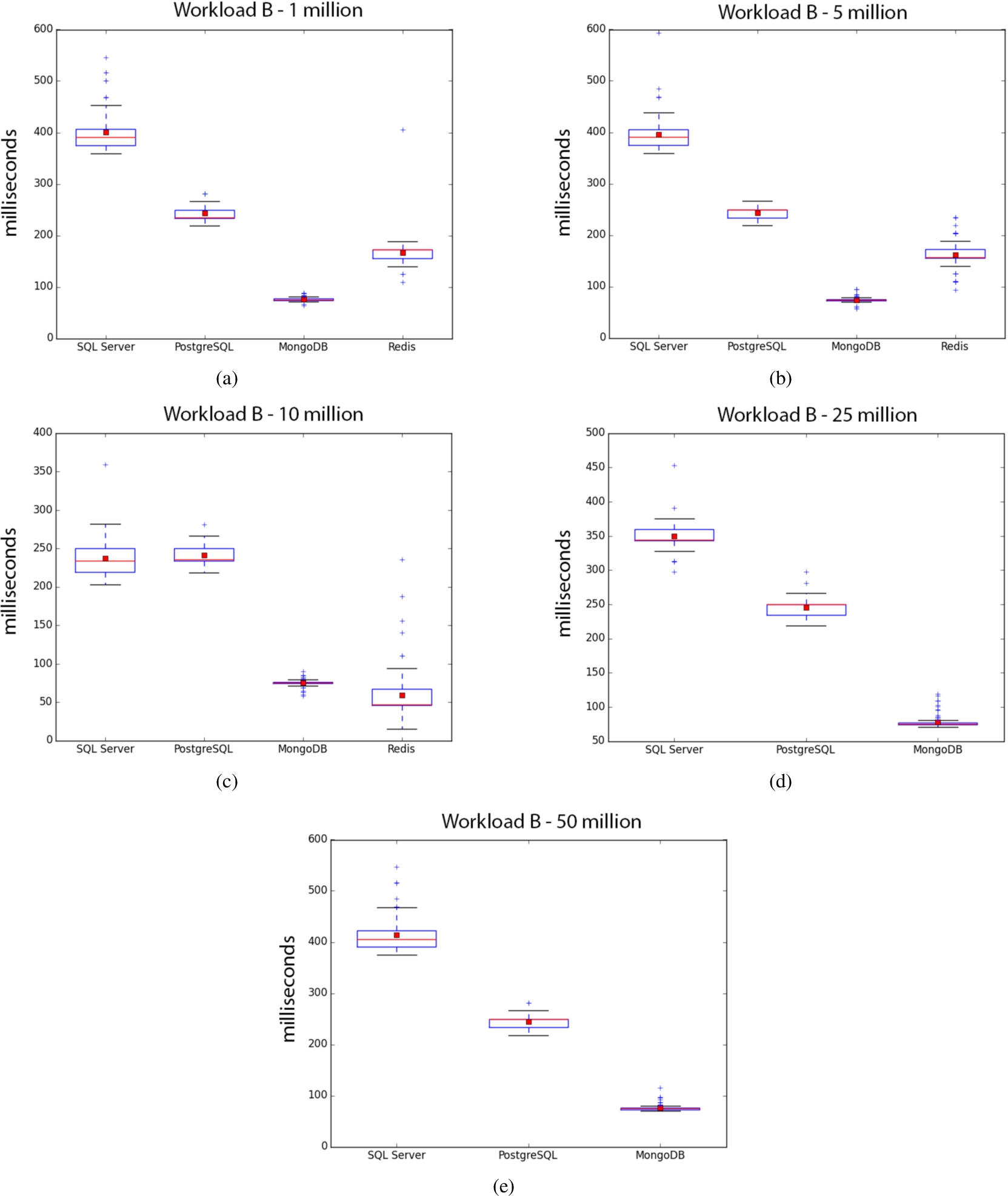
DBMS performance on Workload B.

Fig. 5.

DBMS performance on Workload C.

Tables 8–10 represent time taken to perform the workload B. Figures 4(a)–(e) show the box plots. MongoDB is by far the best, as expected for a test heavily emphasizing reads, consistently beating out everyone else with the exception of Redis at 10 million. Variance at 10 million for Redis is odd, and if viewing the trend from 1 million to 10 million, it looks like it may have continued its poor consistency. SQL Server’s increased performance at 10 million is strange, even with fewer outliers compared to other sizes. However, it was less consistent than PostgreSQL in performance.

6.3. Workload C (100 R)

Table 11
Mean time taken to perform Workload C

Mean (ms) 1 million 5 million 10 million 25 million 50 million

SQL Server 275.31 354.85 234.37 267.03 355.78

PostgreSQL 222.97 223.75 220.47 224.07 220.78

MongoDB 27.37 30.38 28.74 29.58 29.82

Redis 170.47 174.53 78.28

Mean (ms)	1 million	5 million	10 million	25 million	50 million
SQL Server	275.31	354.85	234.37	267.03	355.78
PostgreSQL	222.97	223.75	220.47	224.07	220.78
MongoDB	27.37	30.38	28.74	29.58	29.82
Redis	170.47	174.53	78.28

Table 12

Standard deviation of time taken to perform Workload C

Stddev (ms)	1 million	5 million	10 million	25 million	50 million
SQL Server	95.31	19.73	14.98	79.47	15.61
PostgreSQL	11.52	11.92	12.78	10.29	11.65
MongoDB	4.43	3.34	3.71	3.32	3.04
Redis	10.18	12.75	32.98

Table 13

Mean % speed of to perform Workload C

Mean % speed of	SQL Server	PostgreSQL	MongoDB	Redis
SQL Server	–	75%	10%	47%
PostgreSQL	134%	–	13%	63%
MongoDB	1019%	762%	–	484%
Redis	211%	158%	21%	–

Tables 11–13 represent time taken to perform the workload C. Figures 5(a)–(e) show the box plots. SQL Server variance is very large for the 1 million and 25 million sizes, and not so much on 50 million and 10 million sizes. We get the impression that SQL Server is quite sensitive to something that the other DBMS don’t have. Every size test is run sequentially, so having only SQL Server experience this is strange.

MongoDB takes the lead in both performance and consistency in this read-only test, performing even better than Workload B since it has no writes. PostgreSQL and Redis swap places on who is the most consistent, but when Redis is not around, PostgreSQL places second behind MongoDB, ahead of SQL Server.

6.4. Workload write (100 W)

Tables 14–15 represent time taken to perform the workload Write. Figure 6 shows the box plots. SQL Server is by far the slowest at writes. The test was re-run several times and performance was consistently bad, compared to the other DBMS. PostgreSQL has a strong showing, trailing the MongoDB and Redis slightly. Redis has the best write performance, but not significantly so considering its in-memory advantage. Redis also needs time to write from memory to disk (either at shutdown or at certain time increments), so it could be argued that MongoDB could be placed first overall.

Table 14
Mean time taken to perform Workload Write

Mean (ms) 1000 Inserts

SQL Server 2069.05

PostgreSQL 633.13

MongoDB 465.95

Redis 419.03

Mean (ms)	1000 Inserts
SQL Server	2069.05
PostgreSQL	633.13
MongoDB	465.95
Redis	419.03

Table 15

% speed of to perform Workload Write

% speed of	SQL Server	PostgreSQL	MongoDB	Redis
SQL Server	–	31%	23%	20%
PostgreSQL	322%	–	73%	66%
MongoDB	443%	137%	–	91%
Redis	489%	152%	110%	–

Fig. 6.

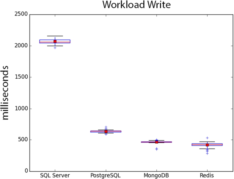
DBMS performance on Workload Write.

6.5. Analysis

SQL Server’s overall performance is not consistent on different workloads. Workload A’s performance was almost uncharacteristically good, and was not repeated for any other workloads. Workload Write’s performance was absolutely abysmal despite identical conditions to other DBMS. We theorize that SQL Server is picky about its running conditions and needs some training or, at the very least, guidance on proper setup to have better performance that default installations won’t provide.

PostgreSQL was consistently average or slightly above average in all tests, making it a predictable and dependable choice. Write performance is also respectable. PostgreSQL appears to be much better suited for different workloads with a default installation, compared to SQL Server.

MongoDB performed extremely well on tests with read requests, even outperforming Redis in many areas. The prerequisite of index creation for reasonable performance on MongoDB shows it not to be a catch-all solution, requiring forward-planning by the developer. Its identical cost to PostgreSQL makes it easy to adopt.

Redis was not much faster in the tests it was best at, and did not end up being first in all tests. It’s likely that Redis needs more finesse in setup to get the most performance out of it. There were no special actions performed on Redis compared to MongoDB (index creation) and with the variety of data structures Redis provides (sorted sets may have helped), its performance would most certainly be better with a more experienced user. In retrospect, Redis’ in-memory advantage is great enough that not doing anything except inserting and testing data (as with SQL Server and PostgreSQL) still allows it to be quite fast. The bottleneck in testing for us was having enough memory to properly complete all the tests.

7. Conclusion and future work

In this paper, we compare four popular SQL and NoSQL DBMS on various size datasets from Twitter. In each workload test, it appears that SQL Server, PostgreSQL and MongoDB handle up to 50 million records of data about the same as only 1 million records, with no considerable benefits or penalties in performance. Looking at Redis’ performance at 1, 5, and 10 million tweets, its performance scaling up is uncertain as they appeared to gradually get worse.

As a whole, NoSQL-based systems appear better for faster performance and read-heavy workloads. SQL-based systems remain competitive, but definitely have a non-zero performance deficit while maintaining ACID compliance.

As for answering the original question of “If I want to store and access millions of tweets for myself, which DBMS should I choose?” We would recommend MongoDB. It has a higher learning curve, but for storing and retrieving tweets, its performance is excellent, and its free and open source nature keeps software costs to a minimum. Hardware needs are not special, and is in fact designed specifically with commodity hardware in mind [11].

For future work, testing with better hardware to fit Redis’ 25-million and 50-million-size datasets would enhance comparisons between it and the other DBMS. Queries can also be expanded to be more complex in nature, involving joins and possibly other resource-intensive tasks.

References

E.A.

Abubakar, Performance evaluation of NoSQL systems using YCSB in a resource austere environment, International Journal of Applied Information Systems7(8) (2014). doi:10.5120/ijais14-451229.

Ameya,

Poriya and

Poojary, Type of NoSQL databases and its comparison with relational databases, International Journal of Applied Information Systems5(4) (2013), 16–19.

Benchmarking Top NoSQL Databases, Datastax Corporation, 2013.

Chang,

Dean,

Ghemawat,

W.C.

Hsieh,

D.A.

Wallach,

Burrows,

Chandra,

Fikes and

R.E.

Gruber, Bigtable: A distributed storage system for structured data, ACM Transactions on Computer Systems (TOCS)26(2) (2008), 4. doi:10.1145/1365815.1365816.

Core workloads, https://github.com/brianfrankcooper/YCSB/wiki/Core-Workloads.

DB-Engines ranking, http://db-engines.com/en/ranking.

Dean and

Ghemawat, MapReduce: Simplified data processing in large clusters, Communications of the ACM51(1) (2008), 107–113. doi:10.1145/1327452.1327492.

Han,

Haihong,

Le and

Du, Survey on NoSQL database, in: Pervasive Computing and Applications (ICPCA), 2011 6th International Conference on, IEEE, 2011, pp. 363–366.

Krikorian, New Tweets per second record, and how! https://blog.twitter.com/2013/new-tweets-per-second-record-and-how.

10.

Parker,

Poe and

S.V.

Vrbsky, Comparing NoSQL MongoDB to an SQL DB, in: Proceedings of the 51st ACM Southeast Conference, Article No. 5, 2013.

11.

Production Notes, http://docs.mongodb.org/manual/administration/production-notes/.

12.

Ramanathan,

Goel and

Alagumalai, Comparison of cloud database: Amazon’s SimpleDB and Google’s Bigtable, in: Recent Trends in Information Systems (ReTIS), 2011 International Conference on, 2011, pp. 165–168.

13.

Seismic Waves, https://xkcd.com/723/.

14.

C.J.

Tauro,

Aravindh and

A.B.

Shreeharsha, Comparative study of the new generation, agile, scalable, high performance NoSQL databases, International Journal of Computer Applications (0975–888)48(20) (2012).

15.

The PostgreSQL Global Development Group, http://www.postgresql.org/community/contributors/.

16.

Zillner,

Becker,

Munné,

Hussain,

Rusitschka,

Lippell,

Curry and

A.K.

Ojo, Big data-driven innovation in industrial sectors, 2016, pp. 169–178.

Operating System	Windows Server 2012 R2 Datacenter
CPU	Intel i7-4790 @ 3.60 GHz
Memory	32GB DDR3-1600
SSD	Samsung 850 PRO 256 GB (OS)
SSD	Samsung 840 EVO 250 GB (VMs)

Operating System	Windows 7 Professional SP1 x64
Disk Size	90 GB
Memory	16384 MB
Virtual Processors	4
Virtual machine reserve (resource control)	100