Renewable and non-renewable energy consumption and economic growth in the US: A Markov-Switching VAR analysis

Abstract

We examine the relationship between renewable and non-renewable energy consumption and economic growth in the United States. While the regime-dependent Granger causality test results for the non-renewable energy consumption and economic growth suggest bi-directional causality in both regimes, we cannot validate any causality between renewable energy consumption and economic growth. The US meets its energy demand from non-renewable sources; as such, renewable energy consumption does not seem to affect economic growth. Given the efficiency and productivity of renewable energy investments, we conclude that it is worthwhile to consider renewable energy inputs to replace fossil fuels given potential benefits in terms of global warming and climate change concerns. In this regard, increasing the R&D investments in the renewable energy sectors, increases in productivity and profitability of renewable energy investments are likely to accrue benefits in the long run.

Keywords

Renewable energy energy consumption economic growth Markov-Switching VAR

Introduction

Energy policies can affect economic activity (growth rate), global warming and carbon emissions.¹ Global warming precipitated by increased environmental pollution due to fossil energy consumption has been a concern at national and international levels for a few decades now.² Thus, combating global environmental pollution also has been prioritized by many countries and institutions.³ As such, many efforts are underway to shift energy production/consumption from conventional sources to non-conventional sources through policies and incentives in order to increase renewable energy production and consumption. For example, the European Union has put forth the Renewable Energy Directive with an explicit focus on the environment, which aims to meet 20% of its energy needs with renewable energy sources by 2030.⁴

The relationship between energy consumption and economic growth has attracted the attention of policymakers and academic professionals alike. Ozturk⁵ and Fallahi⁶ showed that the relationship between energy consumption and economic growth entails four hypotheses. The Conservation Hypothesis concerns regulatory policies for the energy sector will have a negative effect on output. On the other hand, the Growth Hypothesis suggests that energy consumption is intimately connected to economic growth and hence a reduction in energy consumption will cause a slowdown in economic growth. The third hypothesis is the Feedback Hypothesis where there is a feedback relationship between energy consumption and economic growth. In this case, a decrease in energy consumption will result in a decrease in economic growth or vice versa. Finally, the Neutrality Hypothesis suggests no relationship between energy consumption and economic growth or that the positive effects cancel the negative effects all together.

The primary objective of this study is to examine the relationship between energy consumption and economic growth for the US by means of a MS-VAR model. While studies in this area usually use nonlinear Granger causality tests, Lütkepohl⁷ emphasized that Granger causality test results may not tell us the complete story regarding any dynamic relationships among the variables. Moreover, it is important to know the responses of one variable to unexpected shocks in another variable in a system specifically for the policy implications. This would give an idea not only about the significance of the response, but its time path and persistence. While Granger causality test results show the dynamic relationship (if any) between energy consumption and economic growth, the impulse-responses provide a picture about the magnitude and the persistence of the responses of economic growth to an unexpected shock in energy consumption (and vice versa). Hence, we examine the nonlinear relationship between energy consumption and economic growth by using not only regime-dependent Granger causality tests but also regime-dependent impulse-response analysis. Second, while the empirical literature has in general focused on the relationship between non-renewable energy (henceforth, NREN) consumption and economic growth, we focus on the relationship between renewable energy (henceforth, REN) consumption and economic growth. To the best our knowledge, this is the first attempt to examine the nonlinear relationship between REN consumption and economic growth for the US specifically via regime-dependent Granger causality and regime-dependent impulse-response analysis. Our empirical results suggest that both energy consumption and economic growth series exhibit regime-switching properties. We also find that the MS-VAR model outperforms the linear VAR model and hence the MS-VAR model better characterizes the relationship between energy consumption and economic growth. Granger causality test and impulse-responses analysis results show that the relationship between energy consumption and economic growth depends on the business cycle.

We focus on the US economy because carbon emission and greenhouse gas emissions are relatively high in the US. World Bank data suggest that the US produced 22% of the world’s carbon emissions in 1990 and this figure increased to 23% in 2000 and then decreased to 16% in 2010 and 15% in 2014. Even if there are significant decreases in carbon emissions in the US between 1990 and 2014, the US still accounts for the second-highest carbon emissions in the world per World Bank data. On the other hand, the US accounted for 15% of total greenhouse gas emissions in the world between 1990–2012.⁸ According to the EIA⁹ report, the US produced 15.2% of the world’s total carbon emissions in 2015 and 14.9% of total emission in 2016. This highlights the importance of the relationship between energy consumption and economic growth in the US as it provides valuable information for policymakers in terms of designing the proper energy and environmental policies.

According to a US Energy Information Administration report,⁹ the costs of renewable energy sources are generally higher than conventional energy costs. Also, renewable energy technologies still require substantial investments. The US Energy Information and Administration defines the Levelized Cost of Electricity as follows:

Levelized cost of electricity (LCOE) represents the average revenue per unit of electricity generated that would be required to recover the costs of building and operating a generating plant during an assumed financial life and duty cycle … . LCOE include capital costs, fuel costs, fixed and variable operations and maintenance (O&M) costs, financing costs, and an assumed utilization rate for each plant type … .

The US Energy Information and Administration (EIA) calculations are based on a 30-year cost recovery period, using weighted average cost of capital (WACC) equal to 4.2%. In reality, a plant’s cost recovery period and cost of capital can vary according to technology and project type. In this regard, Table 1^10,11 is informative with regards to various energy costs with different technologies.^a The results in Table 1 indicate that the renewable energy costs are fairly competitive compared to conventional energy costs. On the other hand, the EIA Monthly Energy Review statistics indicate biomass was the most consumed renewable energy source for the US in 2018.^b Therefore, non-renewable energy sources (such as natural gas) is still cheaper than the most used renewable energy sources.

Table 1.

Estimated total LCOE (including tax credit).^10,11

Non-renewable energy		Renewable energy
Power plant type	Cost (LCOE) – $/Megawatt	Power plant type	Cost (LCOE) – $/Megawatt
CSSS	130	Wind (offshore)	107
CC Natural Gas	43	Solar Thermal	165
Nuclear Plants	93	Biomass	92
		Hydro	39
		Geothermal	37

Source: IEA, Levelized cost and levelized avoided cost of new generation resources in the annual energy outlook, 2018 and 2019.

Even if the non-renewable energy is the most used energy source in the world, there are several problems with non-renewable energy sources such as environmental impacts, scarcity, supply risks, and instability of prices and markets.^12,13 The instability of fossil resource markets and prices also cause problems in exclusive reliance on these energy resources. As a result, one would expect negative economic consequences.¹³ Countries with high dependence on energy (net energy importers) are extremely sensitive to volatility in fossil energy prices and supplies. When the differences in the supply and demand regions of energy such as oil and natural gas are taken into consideration, energy supply security is a significant concern. Throughout history, energy supplies have been used as a tool in disputes between countries which elevates geopolitical risks.

Figure 1 shows the share of NREN and REN consumption in the total energy consumption in the US between 1949 and 2017. According to the data in Figure 1, while the share of NREN consumption in total energy consumption was up to 90% until the 1980s, the NREN consumption has gradually decreased since at the beginning of the 1980s. The ratio of NREN consumption to total consumption has reached the lowest level in 2017 over the sample. Moreover, the ratio of consumption of REN to total consumption followed a horizontal trend until the mid-1970s, and recorded an upward trend thereafter for six year possibly due to the oil crisis in 1973. Finally, REN consumption has increased significantly since 2001 and the share of REN consumption in total consumption has exceeded 10% for the first time as of 2011.

Figure 1.

Ratio of NREN and REN consumption in total energy consumption.Source: The US Energy Information and Administration.

With differential costs and benefits for renewable and non-renewable energy in the US, and given renewable energy depends on costs of procuring it, it is important to analyze the constraints imposed on te economy by different types of energy. This paper intends to fill a vacuum by analyzing the nonlinear relationship between energy consumption and economic growth for the US specifically via regime-dependent Granger causality and regime-dependent impulse-response analysis. The rest of the paper is organized as follows. We present the literature review in the next section and then econometric framework is presented. We present the empirical results in the Data and empirical results section and finally conclusions are provided.

Literature review

Early work on the relationship between energy consumption and economic growth include Kraft and Kraft¹⁴ where they documented economic growth Granger causes energy consumption. Since then several papers investigated the causality relationship between energy consumption and economic growth in the literature with contradictory results: These were due, among other factors, to different countries, sample periods and econometric models. For example, Cheng¹⁵ found mixed causality relationships between energy consumption and economic growth for Brazil, Mexico, and Venezuela. While there was a causality relationship going from energy consumption to economic growth in Brazil, the study could not validate a causality relationship for Mexico and Venezuela. Masih and Masih¹⁶ found no relationship between energy consumption and economic growth in Malaysia, Singapore, and the Philippines, but Masih and Masih¹⁷ and Asafu-Adjaye¹⁸ found a causality relationship between energy consumption and economic growth in Korea. Glasure,¹⁹, Hondroyiannis et al.²⁰ and Soytas and Sari²¹ found bi-directional causality between energy consumption and economic growth in Korea, Greece and Turkey.

On the other hand, there is a large body of literature examining the relationship between energy consumption and economic growth for the US. For example, Akarca and Long,²² Yu and Hwang²³ and Yu and Jin²⁴ could not find evidence favoring any causality between the energy consumption and economic growth. However, Abosedra and Baghestani²⁵ and Stern²⁶ documented evidence of causal link from the energy consumption to economic growth for the post-war period. Glasure and Lee²⁷ found evidence of bidirectional causality between energy consumption and employment while Zarnikau²⁸ and Lee²⁹ found a similar relationship between energy consumption and economic growth. Chiou-Wei et al.³⁰ extended the literature by employing both the linear and nonlinear Granger causality tests and could not find any causality relationship between variables for the US. Balke et al.³¹ analyzed the effects of oil supply and demand shocks on economic activity for the US and found oil supply and demand shocks affected both the volatility of oil prices and US output. Bowden and Payne³² found unidirectional causality relationship from energy consumption to economic growth. Payne³³ and Yildirim et al.³⁴ could not find any evidence of causality between renewable energy consumption and economic growth while Kum et al.³⁵ found bi-directional causality between natural gas consumption and economic growth. Charfeddine³ and Charfeddine et al.³⁶ concluded that renewable energy consumption affects economic growth in the MENA region significantly. Charfeddine³ examined the impact of oil price changes on the growth rate in Qatar and concluded that energy consumption affects the growth rate positively. Kahia et al.³⁷ found bidirectional causality between renewable energy use and economic growth for the MENA region. Charfeddine et al.³⁸ examined the impact of oil price changes on US growth rate. They find that oil price measures affected growth rate in the first regime (until 1984) and there is no significant effect in the second regime (after 1984). Erdoğan et al.² found that there is a causality from energy consumption to growth for BRICS-T countries. Yıldırım et al.³⁹ found that there is a bi-directional causality relationship between energy consumption and economic growth in BRICS-T countries. Chen et al.⁴⁰ examined the relationship between renewable energy consumption and economic growth. They showed that renewable energy consumption has no significant effect in developed countries and a positive effect on economic growth in OECD countries. Vural⁴¹ found renewable and non-renewable energy consumptions have a significantly positive effect on the growth rate in Sub-Saharan African countries. Alam and Murad⁴² found a unidirectional effect for OECD countries where economic growth affects renewable energy consumption. Le et al.⁴³ examined the effects of renewable and non-renewable energy consumption on the growth rate for 102 countries. They found renewable and non-renewable energy consumption has a significantly positive effect on economic growth. Rahman and Velayutham,⁴⁴ found that renewable and non-renewable energy consumption has significantly positive effect on growth rate in five South Asian countries Musah et al.⁴⁵ examined the link between carbon emissions, renewable energy consumption, and economic growth for West Africa countries. They concluded that renewable energy consumption has no effect on the growth rate.

These empirical results point to a complex set of relationships between energy consumption and economic growth that vary across countries and over time, where direction and the nature of the relationship is sensitive to the sample and whether country-based or global factors are involved. Moreover, the literature has generally employed linear models to examine the relationship between energy consumption and economic growth. In the meantime, extensive studies in the literature documented that economic growth exhibits asymmetries depending on the business cycle (expansions vs. contractions). Also, the existence of structural breaks in energy prices, changes in energy policies, extensive regulations in the energy market, and supply and demand shocks in the energy sector can cause asymmetries in energy consumption. Depending on these factors, the relationship between energy consumption and economic growth may be time-varying according to business cycle and under these circumstances, linear models are not appropriate in examining the relationship between energy consumption and economic growth.

There are a limited number of studies investigating the relationship between energy consumption and economic growth using nonlinear models. For example, Lee and Chang⁴⁶ and Hu and Lin⁴⁷ employed a threshold model to examine the energy consumption and economic growth for Taiwan. Fallahi⁶ and Kocaaslan⁴⁸ examined the relationship between non-renewable energy consumption and economic growth by using a regime-dependent Granger causality test that depends on Markov-Switching Vector Autoregressive (MS-VAR) model. On the other hand, Mezghani and Haddad⁴⁹ emphasized the importance of the time-varying relationship between GDP, non-renewable energy consumption and CO2 emissions and hence employed Time-Varying Parameter Vector Autoregressive (TVP-VAR) model to examine the relationship between the variables. Bildirici and Gokmenoglu⁵⁰ investigated the relationship between hydroelectric energy consumption, economic growth and environmental pollution with a regime-dependent Granger causality test. The empirical results of these studies confirmed nonlinearities and the relationship between energy consumption and economic growth is nonlinear in nature.

Econometric framework

There is a well-documented literature that the US real GDP has regime-switching properties (e.g. see Hamilton⁵¹; Kim and Nelson⁵²; Krolzig⁵³; Camacho⁵⁴; Charfeddine et al.³⁸). Moreover, Hamilton⁵¹ and Krolzig⁵³ showed that the Markov-Switching model provides better forecast performance than linear models for the US GDP. On the other hand, there is scant attention paid to nonlinearity in energy consumption. Therefore, it is important to examine whether the energy consumption series has nonlinear dynamics before attempting to estimate nonlinear models.

Linearity test

A Likelihood Ratio (LR) test is commonly employed in the literature to ascertain whether the Markov-Switching model is a better fit for the data. The LR test statistic is given by:

L R = 2 [L (θ) - L (θ_{r})]

(1)

where L(θ) and L(θ_r) are the log-likelihood values for the Markov-Switching model and the linear model respectively and r represents the number of restrictions. The LR test follows a χ² distribution with r degrees of freedom. However, following conventional procedures for testing the Markov-Switching model is complicated because the transition probabilities in the Markov-Switching model are not defined in the linear model and hence the asymptotic distribution does not follow a standard χ²-distribution. To handle this problem, we use upper bond p-values suggested by Davies.⁵⁵

Even though the LR test has been extensively used in the literature, a limited number of studies analyze nonlinearity in energy consumption data in the literature. Therefore, a Markov-Switching specific test must be employed to ascertain regime-switching properties in energy consumption. There are several Markov-Switching specific linearity tests in the literature (See Hansen⁵⁶; Garcia⁵⁷; Cho and White⁵⁸ and Carrasco et al.⁵⁹) Di Sanzo⁶⁰ suggested a test procedure for Markov-Switching models based on a bootstrap resampling procedure and using Monte Carlo simulations, showed that bootstrap resampling has better performance than the test proposed by Hansen⁵⁶ and Carrasco et al.⁵⁹ Di Sanzo⁶⁰ showed this test does not require extensive computations and gives better results in small samples.

The bootstrap based LR test can be implemented using the following four steps. The first step consists of obtaining the standardized residuals for the linear model. In the second step, the LR test defined in equation (1) is used to obtain the log-likelihood values of the linear and Markov-Switching models.^c The bootstrap sample is created by using estimated parameters and bootstrap residuals of the linear model in the third step. In the final step, the LR* test statistic is computed via the bootstrap sample and repeating the steps (3 & 4) 500 times. This way, the distribution of the LR* statistic is obtained and the bootstrap p-value can be calculated as $p_{B} = card (L R * \geq L R) / 500$ that is the fraction of LR* values which are greater than the observed value, LR.

The MS-VAR model

The MS-VAR model proposed by Krolzig⁶¹ is the multivariate generalization of Hamilton’s⁵¹ single Markov-Switching model and it is largely used in the literature to analyze regime-dependent relationships among variables in a system. As in the single Markov-Switching model, the regimes can be defined according to the unobserved state variable that follows a Markov process in the MS-VAR model. Note that all variables are considered endogenous in the MS-VAR model and the dynamic relationship among the variables can be analyzed by means of Granger causality tests and impulse-response functions over the regimes.

Consider y_t as a T x 1 vector including endogenous variables and let Y_t = (y_1t, y_2t, … , y_Kt), t = 1, 2, … , T be K-dimensional time series vector, where T is the sample size. Then, a p-th order and m state MS-VAR model can be written as:

Y_{t} = {\begin{cases} v_{1} + A_{11} Y_{t - 1} + \dots + A_{p 1} Y_{t - p} + B_{1} u_{t} if s_{t} = 1 \\ ⋮ \\ v_{m} + A_{1 m} Y_{t - 1} + \dots + A_{p m} Y_{t - p} + B_{m} u_{t} if s_{t} = m \end{cases}

(2)

In equation (2), v_i are constant terms and A_1i, … , A_pi are autoregressive coefficient matrices for VAR parameters corresponding to states. The matrices B₁u_t are the reduced-form shocks, and u_t follows a multivariate normal distribution. N (0, I_K) and the regime-dependent variance-covariance matrix for the residuals can be formulated as follows:

\sum_{i} = E (B_{i} u_{t} u_{t}^{'} B_{i}^{'}) = B_{i} E (u_{t} u') B_{i}^{'} = B_{i} I_{K} B_{i}^{'} = B_{i} B_{i}^{'}

(3)

The transition process of the Markov-Switching model is given by a first-order m state Markov stochastic process. Let p_ij be transition probability that state i in period t will be followed by state j in period t + 1, which is defined as;

p_{i j} = P (s_{t + 1} = j / s_{t} = i), \sum_{j - 1}^{m} p_{i j} = 1 \forall i, j \in (1, \dots, m)

(4)

In addition, all transition probabilities can be defined as an m x m transition matrix as follows:

[\begin{matrix} p_{11} & p_{12} & \dots & p_{1 m} \\ p_{21} & p_{22} & \dots & p_{2 m} \\ ⋮ & ⋮ & ⋱ & ⋮ \\ p_{m 1} & p_{m 2} & \dots & p_{m m} \end{matrix}]

(5)

The MS-VAR model is a nonlinear model in nature, hence, the regime parameter s_t is unobservable and maximum likelihood methods must be used to estimate the parameters. As such we use the Maximum Likelihood (ML) method based on the Expectation-Maximization (EM) algorithm to estimate the parameters. This iterative technique obtains both the estimates of the parameters and the transition probabilities governing the Markov chain of the unobserved states.

Kanas and Ionnidis⁶² suggested the causality between variables in the MS-VAR model can be tested by a Likelihood Ratio (LR) test where the causal link is examined by imposing restrictions for the estimated autoregressive coefficients in each regime. The LR test statistic follows a χ² (k) distribution asymptotically where k is number of restrictions.

The impulse-response functions proposed by Ehrmann et al.⁶³ can also be considered to best understand the dynamic relationships between energy consumption and real GDP. Calculating impulse-response functions in the MS-VAR model requires estimating the regime-dependent variance-covariance matrices (such as ∑₁, … ∑₂ , …, ∑_m). Note that Ehrmann et al.⁶³ used Cholesky decompositions to identify the shocks in the regime-dependent impulse-responses functions because the number of estimated parameters in the reduced-form model must be less than the structural model in the MS-VAR.

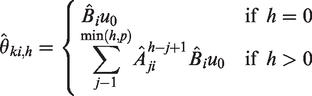
When one standard deviation shock to the variable k occurs at time t in the regime i, the regime-dependent impulse-responses at time t + h can be described as follows:

[\frac{\partial E_{t} R_{t + h}}{\partial u_{k, t}} | (S_{t} = \dots S_{t + h} = i)] = θ_{k i, h,} h = 0, 1, 2, \dots

(6)

Ehrmann et al.⁶³ generalized the regime-dependent impulse-response functions as:

{\hat{θ}}_{k i, h} = {\begin{array}{l} {\hat{B}}_{i} u_{0} & if h = 0 \\ \sum_{j - 1}^{\min (h, p)} {\hat{A}}_{j i}^{h - j + 1} {\hat{B}}_{i} u_{0} & if h > 0 \end{array}

Data and empirical results

We examine the possible regime-dependent relationship between energy consumption and economic growth for the US for 1973Q1-2019Q4. We consider both REN and NREN energy consumption and analyze the relationship between two measures of energy consumption and economic growth. NREN energy consumption is the sum of coal, natural gas and oil consumption and is measured in quadrillion BTUs. Renewable energy consumption is the sum of Hydroelectric Power, Geothermal Energy, Solar Energy, Wind Energy, and Biomass Energy in quadrillion BTUs. We also consider per capita carbon emissions (CO2) and financial development (henceforth, FD) as a control variable in the model estimations. As in Charfeddine and Kahia,⁶⁴ financial development is calculated as the ratio of private sector credit to GDP. The data on energy consumption and carbon emissions are obtained from the US Energy Information and Administration (EIA) and real GDP and FD series are taken from the Federal Reserve Bank of Saint Louis FRED database. We use Tramo/Seats to adjust for seasonal effects in the data and express the series in natural logarithms.

Real GDP for the US is presented in Figure 1. The figure shows that the US experienced two extensive growth periods in the recent decades. One was fueled by the information technology revolutions of the 1990 and the more recent one was due to massive stimulating monetary/fiscal policy measure undertaken post 2007–2009 financial crisis. The US economy is currently undergoing a severe shock due to the Covid-19 global health pandemic in the first half of 2020. Even though it is too early to assess the comprehensive effect on the economy, global oil prices collapsed and for the first time in history, on April 20, 20202 the 1-month West Texas Intermediate futures contract traded in the negative territory^d due to concerns of an increase in supply to the market, a saturation of storage capacity, and low demand in addition to the Covid-19 pandemic. This decrease in conventional energy is likely to negatively affect renewable energy production given the unusually low price for conventional sources of energy based on fossil fuels in the current climate (Figure 2).

Figure 2.

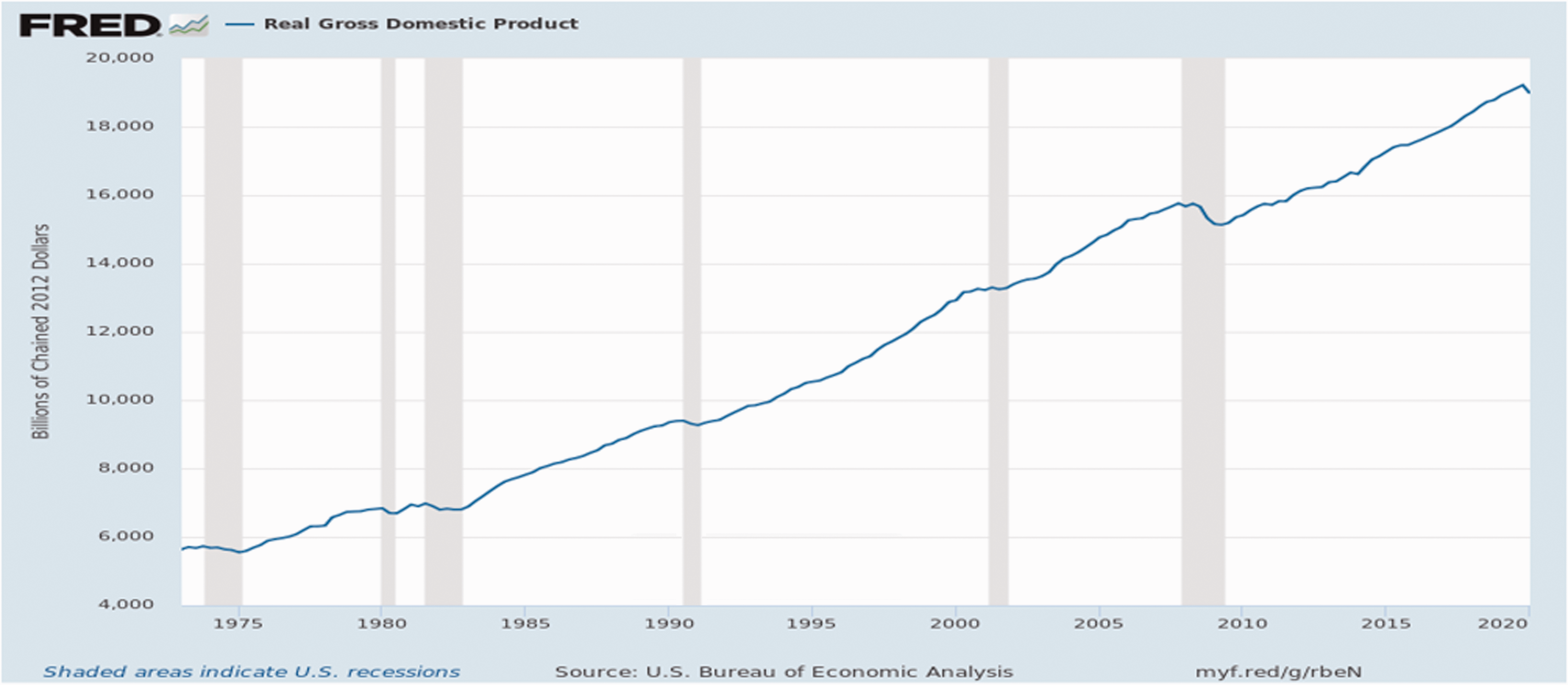
The real GDP.

We start our analysis by testing for unit roots. To that end, we run Augmented Dickey-Fuller (henceforth, ADF) and Phillips-Perron (henceforth, PP) unit root tests; we present results in Table 2. According to the test results, we cannot reject the null hypothesis of a unit root in levels for all variables at conventional significance levels. On the other hand, the null hypothesis is rejected at the 1% significance level when we consider first differences of the series.

Table 2.

Unit root test results.

Variables	Level		First differences
Variables	ADF	PP	ADF	PP
REN	–1.984	–1.723	–9.023***	–12.672***
NREN	–1.591	–2.169	–6.044***	–16.251***
GDP	–0.949	–1.276	–4.543***	–9.723***
CO2	–1.542	–2.056	–6.079***	–16.140***
FD	–2.036	–1.380	–3.269***	–8.676***

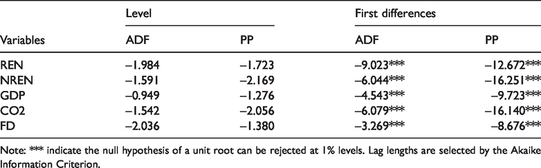
Note: *** indicate the null hypothesis of a unit root can be rejected at 1% levels. Lag lengths are selected by the Akaike Information Criterion.

It is well known that the conventional unit root tests have low power to reject the null hypothesis when there are structural breaks in the series. Therefore, we also employ unit root test with structural breaks suggested by Kapetanios.⁶⁵ The null hypothesis of unit root is tested against alternative of stationarity with k unknown breaks. We employ unit root test that allows to change in intercept up to 5 breaks and present the results in Table 3.^e The results in Table 3 show that the null hypothesis of unit root cannot be rejected at conventional level for all series. Both types of unit root tests result with or without structural breaks indicate that it is appropriate to consider first differences of variables in the econometric analyses.

Table 3.

Unit root test with structural breaks results.

Variables		Number of breaks
Variables		k = 1	k = 2	k = 3	k = 4	k = 5
NREN	Test Statistic	–2.826	–2.099	–2.278	–2.737	–3.005
NREN	Break Dates	1983Q1	1978Q2- 1983Q1	1978Q2- 1983Q1- 2007Q3	1978Q2- 1983Q1- 1933Q2- 2007Q3	1978Q2- 1983Q1- 1987Q4- 1933Q2- 2007Q3
REN	Test Statistic	–3.319
REN	Break Dates	1984Q2
GDP	Test Statistic	–3.652	–4.102	–4.925	–5.276	–5.737
GDP	Break Dates	2007Q4	1982Q3- 2007Q4	1982Q3- 1997Q1- 2007Q4	1982Q3- 1991Q4- 1997Q1- 2007Q4	1982Q3- 1991Q4- 1997Q1- 2003Q1- 2007Q4
CO2	Test Statistic	–2.939	–2.277	–2.398	–2.76	–3.033
CO2	Break Dates	1983Q1	1978Q2- 1983Q1	1978Q2- 1983Q1- 2007Q3	1978Q2- 1983Q1- 1994Q4- 2007Q3	1978Q2- 1983Q1- 1987Q4- 1994Q4- 2007Q3
FD	Test Statistic	–3.079	–3.317	–1.867	–2.347	–2.461
FD	Break Dates	2007Q4	1986Q4- 2007Q4	1986Q4- 2001Q1- 2007Q4	1981Q4- 1986Q4- 2001Q1- 2007Q4	1981Q4- 1986Q4- 1993Q1- 2001Q1- 2007Q4
CV 1%		−5.338	−6.162	−6.991	−7.560	−8.248
CV 5%		−4.930	−5.685	−6.529	−7.104	−7.636
CV 10%		−4.661	−5.467	−6.265	−6.832	−7.398

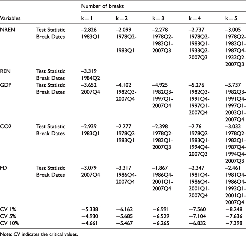
Note: CV indicates the critical values.

Linearity test results

We first examine whether the MS-VAR model better characterizes the relationship between energy consumption and economic growth than a linear model using model selection criteria. First, we estimate a two-state MS-VAR model^f with four variables (GDP growth, financial development growth, growth in CO2 and NREN/REN consumption growth) and present model information criteria in Table 4.^g According to results in Table 4, the Akaike information criterion suggests the MS-VAR model in modelling the relationship between energy consumption and economic growth over the sample. Furthermore, Davies p-value provides strong evidence in favor of the MS-VAR model because the null hypothesis of the linear VAR model is rejected at the 1% significance level.

Table 4.

Model information criteria and LR test results.

	NREN		REN
	MS-VAR	Linear VAR	MS-VAR	Linear VAR
Log-likelihood	2355.159	2284.651	1886.756	1834.154
AIC	–24.445	–24.201	–19.621	–19.399
BIC	–22.808	–23.401	–18.548	–18.897
HQ	–23.781	–23.877	–18.545	–18.897
Davies p-value	0.000		0.000
Di Sanzo p-value	0.040		0.071

Note: AIC, BIC, and HQ indicate Akaike, Bayesian Schwarz and Hannan-Quinn information criterions respectively.

We also conduct a Markov-Switching specific test suggested by Di Sanzo⁶⁰ to ascertain nonlinearity in the relationships. The null hypothesis of no regime-switching is tested against the alternative of a two-state Markov-Switching model in the LR test. The bootstrap p-value for the LR test is given in Table 4. The results in Table 4 show that the null hypothesis of no regime-switching can be rejected at the 5% significance level for REN consumption and at the 10% significance level for NREN consumption.^h These results favor regime dependence/switching in measures of energy consumption and thus, a two-state MS-VAR model seems to be more appropriate to model the relationship between energy consumption and economic growth.

The relationship between non-renewable energy consumption and economic growth

The two-state MS-VAR model results for the NREN and economic growth are presented in Table 5. The optimum lag length is decided on the basis of Akaike information criterion (AIC) in the MS-VAR model where the AIC suggests 2 lags are adequate to make residuals approximately white noise. We present parameter estimates in four panels in Table 5 where Panel A and Panel B show regime transition matrix while Panel C gives information on regime properties. Finally, model diagnostics test results are presented in Panel D. The estimated smoothed transition probabilities that are obtained from the MS-VAR model for Regime 1 are presented in Figure 3.

Table 5.

MS-VAR model results for non-renewable energy consumption.

	Regime 1 (Recession)				Regime 2 (Expansion)
	FD_t	GDP_t	NREN_t	CO2_t	FD_t	GDP_t	NREN_t	CO2_t
Constant	0.0002 [0.925]	–0.003 [0.360]	–0.020*** [0.000]	–0.100*** [0.000]	0.001 [0.172]	0.006*** [0.000]	–0.006 [0.109]	–0.046*** [0.009]
FD_t-1	0.258 [0.179]	–0.060 [0.790]	–0.070 [0.842]	0.221 [0.900]	0.288*** [0.000]	0.117 [0.022]	0.034 [0.876]	–0.073 [0.945]
FD_t-2	0.110 [0.586]	–0.076 [0.763]	–0.378 [0.305]	–2.338 [0.212]	0.513*** [0.000]	–0.063 [0.203]	–0.039 [0.857]	0.262 [0.801]
GDP_t-1	0.018 [0.908]	0.418** [0.029]	0.526* [0.071]	2.368 [0.107]	–0.122 [0.225]	0.182** [0.017]	0.852*** [0.000]	4.077*** [0.008]
GDP_t-2	–0.171 [0.300]	0.110 [0.576]	0.990*** [0.001]	5.317*** [0.001]	0.024 [0.787]	0.090*** [0.000]	0.230 [0.406]	0.981 [0.469]
NREN_t-1	0.135 [0.747]	1.546** [0.012]	0.343 [0.653]	3.740 [0.334]	0.034 [0.821]	–0.220** [0.039]	0.369 [0.428]	2.589 [0.245]
NREN_t-2	–0.221 [0.603]	0.792 [0.169]	1.229 [0.109]	6.268 [0.107]	0.001 [0.994]	–0.268** [0.010]	–0.308 [0.471]	–0.548 [0.793]
CO2_t-1	–0.055 [0.538]	–0.340** [0.016]	–0.123 [0.445]	–0.922 [0.259]	–0.004 [0.880]	0.051** [0.019]	–0.151 [0.116]	–0.859* [0.062]
CO2_t-2	0.067 [0.459]	–0.178 [0.154]	–0.376** [0.021]	–1.775*** [0.031]	0.005 [0.849]	0.058*** [0.007]	0.018 [0.840]	–0.069 [0.874]
σ	0.008	0.010	0.015	0.078	0.006	0.004	0.018	0.089
	Panel B: Transition Matrix
		Regime 1					Regime 2
Regime 1		0.816					0.184
Regime 2		0.041					0.959
	Panel C: Regime Properties
		Observation Number				Probability		Duration
Regime 1		37.1				0.182		5.43
Regime 2		147.9				0.817		24.33
	Panel D: Diagnostics Test
P-χ²		236.438
N- χ²		7.437
H- χ²		130.590

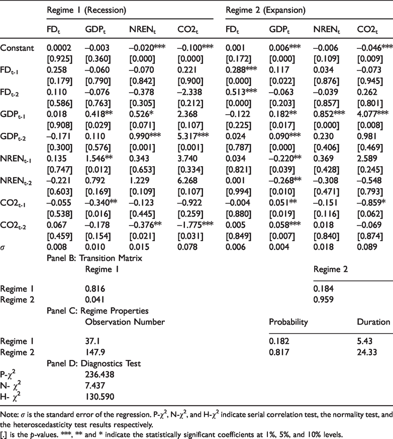
Note: σ is the standard error of the regression. P-χ², N-χ², and H-χ² indicate serial correlation test, the normality test, and the heteroscedasticity test results respectively. [.] is the p-values. ***, ** and * indicate the statistically significant coefficients at 1%, 5%, and 10% levels.

Figure 3.

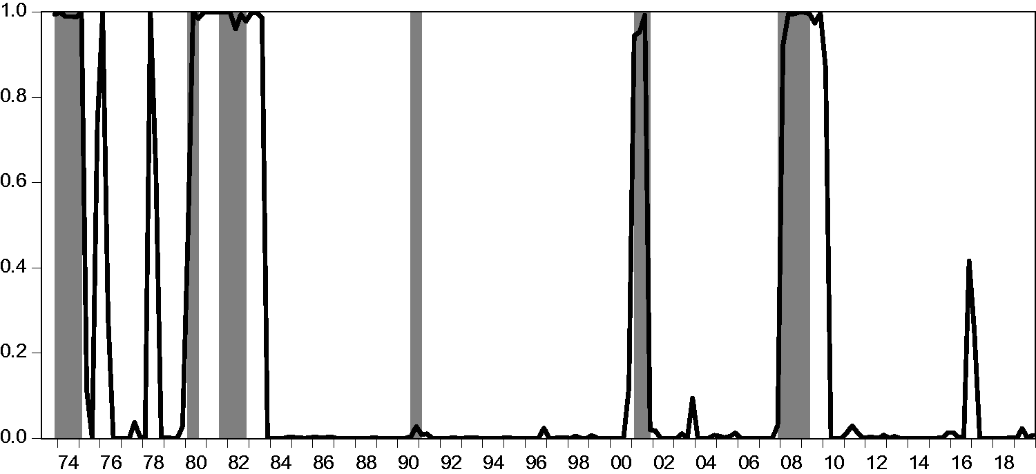
The smoothed probabilities for regime 1.Note: Shaded areas indicate the NBER recessions.

In order to identify the regimes properly, we consider the estimated smoothed probabilities, a method widely used in the literature. The estimated smoothed probabilities for Regime 1 track NBER recessions well. This suggests that Regime 1 can be identified as the “recessions regime” and Regime 2 can be considered as the “expansion regime.” The results in Panel B and Panel C of Table 5 show regime properties where the expansion regime is more persistent than the recession regime over the sample. According to the transition matrix, the probability of remaining in an expansion if the economy is already in an expansion regime is 95.9% whereas the probability of remaining in a recession if the economy is already in a recession is 81.6%. The regime properties in Panel C indicate that the mean duration of expansion and recession regimes is 24.33 and 5.43 quarters respectively and this is not too far from the actual observed business cycles in the US^54,i

In order to examine any causality relationship between NREN consumption and real GDP, we use a regime-dependent Granger causality test by imposing restrictions on the autoregressive coefficients in the MS-VAR model and results are given in Table 6.^j The Granger causality test results indicate a bidirectional causality between NREN consumption and economic growth in both regimes. These results provide evidence in favor of the feedback hypothesis for the relationship between NREN consumption and economic growth in the US. This finding is consistent with the empirical results documented in Glasure and Lee,²⁷ Zarnikau²⁸ and Lee.²⁹

Table 6.

Regime-dependent Granger causality test results.

Causality relationship	Recession		Expansion
GDP → NREN	18.640***	[0.000]	10.446***	[0.005]
NREN → GDP	6.692**	[0.035]	10.831***	[0.004]

Note: The figures in square brackets show the probability (p-values) of rejecting the null hypothesis. *** and ** indicate causal relationship at the 1% and 5% significance level respectively.

On the other hand, the causality relationship tends to vary from recessions to expansions. For example, although the null hypothesis of no causal link from NREN to real GDP consumption can be rejected at the 5% significance level in recessions, it can be rejected at the 1% significance level in the expansion regime. However, the causal link from real GDP to NREN consumption is statistically significant at the 1% level in both regimes.

A remaining important question is the magnitude and the persistence of the responses of economic growth to unexpected shocks in energy consumption (and vice versa). Here, we present regime-dependent impulse-response functions and the results are given in Figure 4.^k,l The results in the top of Figure 4 show the responses of real GDP to an unexpected shock in the NREN consumption over the regimes whereas the responses of NREN consumption to a real GDP shock are presented at the bottom of the Figure. According to the results in Figure 4, although the real GDP reacts first positively (but not statistically significant) to a shock NREN consumption in the recessions, it turns to be negative and statistically significant in the second and third quarter. On the other hand, the response of real GDP to a NREN consumption shock is positive and statistically significant in the expansion.

Figure 4.

Impulse responses analysis results for NREN and GDP.Note: Dashed lines indicate standard error confidence intervals.

These results suggest that the responses of the real GDP to an NREN consumption shock are different under different regimes where real GDP reacts immediately to a NREN consumption shock in both regimes but the reaction is significant only in the expansion regime. These results are consistent with what one would expect since NREN is one of the primary energy inputs in the production process and hence it an increase in demand for energy in the production process leads to increase economic growth immediately when the economy is in expansion. On the other hand, when output is on a stagnation trajectory, an increase in demand for energy in the production process does not immediately affect economic growth. While real GDP reacts immediately to an unexpected shock in NREN consumption in expansions, the responses of real GDP seems to accommodate a shock in the NREN consumption in recessions. Given many studies that document a relationship between oil price shocks as a driving force behind US business cycles in the post-war period, one can attribute the immediate effect of energy consumption on economic growth in expansions, to possible increases in energy prices.^67,68 The same effect seems to work also in recessions; however, it seems to be weak initially.

According to results in Figure 4, although NREN reacts first positively and statistically significant to a shock real GDP in the recessions, it turns to be statistically significant after the second quarter. Note that the standard errors of the responses are generally borderline cases. On the other hand, the NREN consumption reacts negatively but not statistically significant to a shock real GDP in the expansions, which turns to be positive and statistically significant in the first and third quarter.

The relationship between renewable energy consumption and economic growth

The two-state MS-VAR model results for REN consumption and economic growth are presented in Table 7. Optimum lag lengths are selected by AIC indicates one lag is adequate to render residuals white noise. The studies in the literature generally use the estimated parameters and/or comparing the states to a specific set of dates that establish the timing of shifts between regimes.^m The smoothed transition probabilities for Regime 1 presented in Figure 5 reasonably match NBER recessions and hence we identify Regime 1 as a recession regime.

Table 7.

MS-VAR model results for renewable energy consumption.

	Regime 1 (Recession)						Regime 2 (Expansion)
	FD_t		GDP_t		REN_t	CO2_t	FD_t		GDP_t	REN_t		CO2_t
Constant	0.001 [0.243]		0.003* [0.078]		0.001 [0.946]	–0.049*** [0.005]	0.003** [0.039]		0.006*** [0.000]	0.008 [0.176]		–0.031* [0.064]
FD_t-1	0.165 [0.262]		–0.041 [0.840]		0.099 [0.905]	0.962 [0.623]	0.667*** [0.000]		0.092** [0.010]	–0.565** [0.047]		–0.138 [0.862]
GDP_t-1	0.029 [0.780]		0.366** [0.018]		0.573 [0.345]	3.580** [0.017]	–0.152 [0.266]		0.113 [0.165]	–0.165 [0.788]		3.884** [0.041]
REN_t-1	–0.024 [0.302]		0.018 [0.594]		0.141 [0.293]	0.402 [0.213]	–0.054*** [0.007]		–0.011 [0.315]	–0.007 [0.932]		–0.151 [0.540]
CO2_t-1	–0.008 [0.444]		0.014 [0.369]		–0.131** [0.037]	–0.176 [0.231]	0.001 [0.941]		0.006 [0.116]	–0.057* [0.060]		–0.243*** [0.005]
σ	0.008		0.011		0.015	0.104	0.007		0.004	0.018		0.089
		Panel B: Transition Matrix
				Regime 1							Regime 2
Regime 1				0.895							0.105
Regime 2				0.037							0.963
		Panel C: Regime Properties
				Observation Number				Probability		Duration
Regime 1				54.4				0.261		9.56
Regime 2				131.6				0.738		26.98
		Panel D: Diagnostics Test
P-χ²				318.550
N- χ²				6.269
H- χ²				60.767

Figure 5.

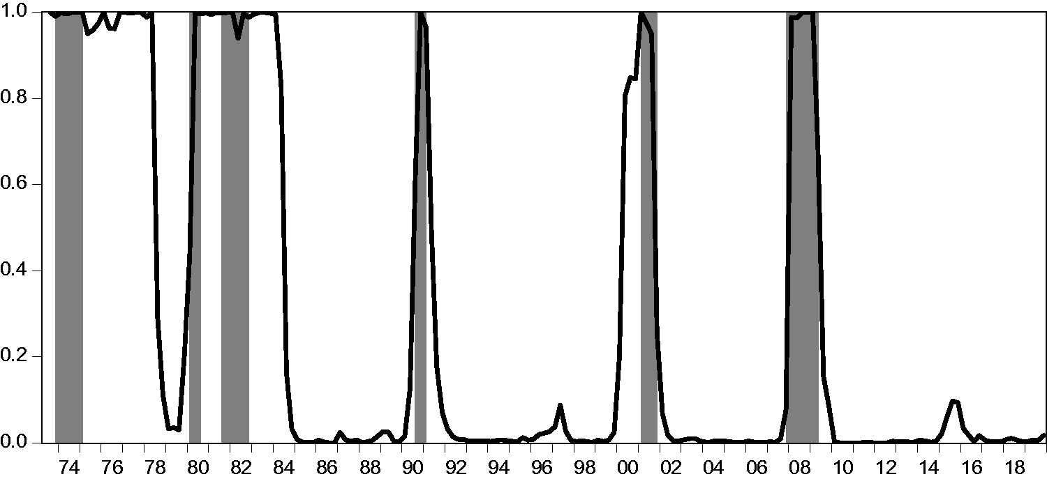
The smoothed probabilities for regime 1.Note: Shaded areas indicate the NBER recessions.

The results in Panel B and Panel C of Table 7 show that the expansion regime is more persistent than the recession regime over the sample. According to the transition matrix, the probability of remaining in an expansion if the economy is already in an expansion regime is 96.3% whereas the probability of remaining in a recession at time t when the economy is also in a recession regime at time t-1 is 89.5%. According to regime properties results in Panel C, the mean duration of expansion and recession regimes are 26.98 and 9.56 quarters respectively.

The regime-dependent Granger causality test results are presented in Table 8. We cannot validate any causal link between REN consumption and the economic growth in either regime and these results provide evidence in favor of the Neutrality hypothesis in terms of renewable energy consumption and economic growth in the US. These results are consistent with empirical results found in Payne³³ and Yildirim et al.³⁴ It is possible that the consumption of renewable energy is not widespread so as to constrain economic growth or vice versa.

Table 8.

Regime-dependent Granger causality test results.

Causality relationship	Recession		Expansion
GDP → REN	0.899	[0.342]	0.072	[0.787]
REN → GDP	0.286	[0.592]	1.017	[0.313]

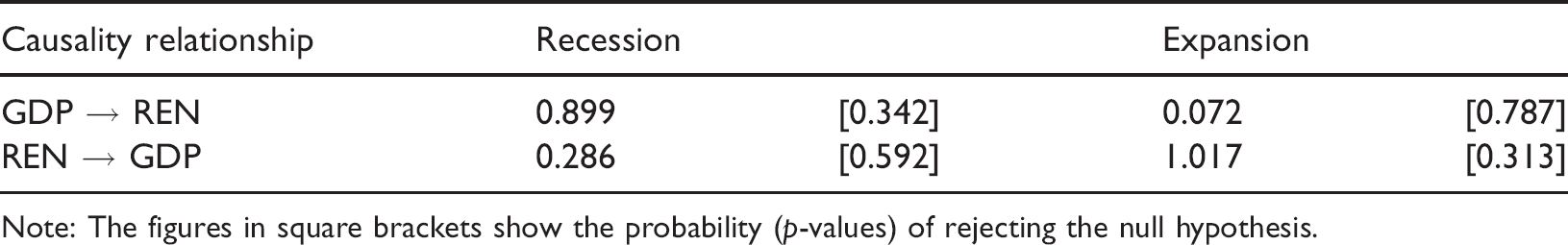
Note: The figures in square brackets show the probability (p-values) of rejecting the null hypothesis.

We finally estimate regime-dependent impulse-responses functions and the results are given in Figure 6. The results indicate that the responses of economic growth to a shock in the REN consumption is not statistically significant in recessions. On the other hand, the responses of economic growth to a shock in REN consumption are negative and statistically significant in expansions. According to these results, an unexpected demand in renewable energy in expansions affects economic growth in the US negatively. This is consistent with the empirical results found in Payne³³ and Bhattacharya et al.⁶⁸ It should be noted that the primary energy input in the production process is still non-renewable energy in the US and renewable energy production is a long-term and relatively costly investment and hence the US is likely to rely on non-renewable energy sources in the near future to ease the constraints on economic growth. We also estimate the responses of REN consumption to economic growth, which are not statistically significant in either regime. These corroborate the Granger causality test results above.

Figure 6.

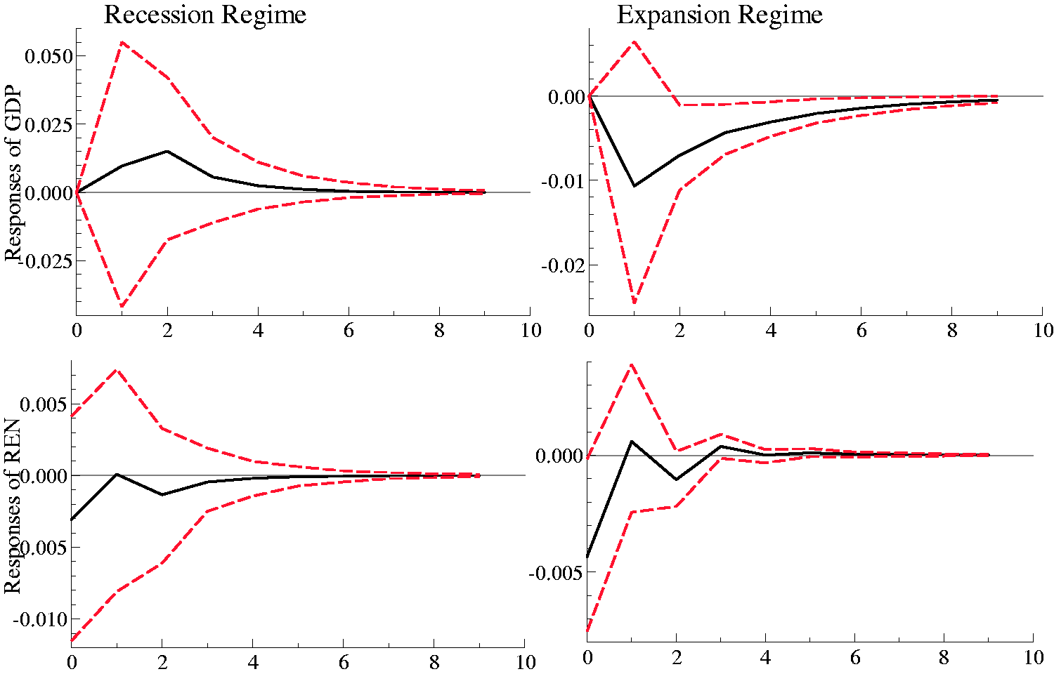
Impulse responses analysis results for REN and GDP.Note: Dashed lines indicate standard error confidence intervals.

Concluding discussion

The relationship between energy consumption and economic growth has been widely discussed in the literature. Carbon emissions resulting from energy consumption often bring attention to the type of energy inputs used in production. Within the framework of the Kyoto Protocol and subsequent agreements, many countries pledged to increase the share of renewable energy inputs in total energy consumption in order to limit the negative effects of energy use given global warming concerns. In this regard, documenting the impact of renewable energy consumption on economic growth is important for policymakers. Identification of the direction and magnitude of the relationship between different types of energy and economic growth provides valuable information for policymakers.

Even though the literature is replete with studies investigating the relationship between energy consumption and growth, the results are not clear cut. This is possibly due to different sample periods and/or countries. Since output tends to exhibit asymmetric behavior over the business cycles, it is important to account for these asymmetries by using non-linear methods. Moreover, the existence of structural breaks in energy prices, changes in energy policies, regulations in the energy market and supply and demand shocks in the energy sector can be a source of asymmetries in energy consumption and its potential effects on output. Therefore, the relationship between energy consumption and economic growth can exhibit nonlinear characteristics and in such a case, linear models provide poor results in assessing the relationship between energy use and output.

In this study, we distinguish between different types of energy consumption and economic growth by considering renewable and conventional energy types for the US. These energy sources vary in their cost and global non-renewable energy supplies exhibit some instability that affect their availability and cost. We consider the US economy as the US accounts for a significant portion of global carbon and greenhouse gas emissions.

Our test results indicate that REN and NREN exhibit regime-switching properties and a MS-VAR model better accounts for the relationship between energy consumption and economic growth over the sample. The two-state MS-VAR model seems to be suited to examine the relationship between energy consumption and economic growth where we identify the regimes as recession and expansion regimes. The Granger causality test results indicate the presence of bidirectional causality between economic growth and NREN consumption in the both regimes and these results lend support to the feedback hypothesis. This is consistent with the empirical results found in Glasure and Lee,²⁷ Zarnikau²⁸ and Lee.²⁹ We cannot find any causal link between REN consumption and real GDP in either regime, and this lends support to the so-called Neutrality Hypothesis. These results are consistent with empirical results found in Payne³³ and Yıldırım et al.³⁴ The regime-dependent impulse-response functions indicate the response of economic growth to REN consumption is not statistically significant in either of the two regimes.

While results suggest bi-directional causality between non-renewable energy consumption and economic growth in this paper, we cannot ascertain significant relationships between renewable energy consumption and economic growth possibly due to limited use of this type of energy in the US. To the extent that the US meets its energy demand from non-renewable sources, renewable energy consumption does not statistically affect economic growth. The neutral effect of renewable energy consumption on economic growth can be explained by its limited use. Given the efficiency and productivity of renewable energy investments, it is worthwhile to consider renewable energy inputs to replace fossil fuels given potential benefits in terms of global warming and climate change concerns. In this regard, increasing the R&D investments in the renewable energy sectors, increases in productivity and profitability of renewable energy investments are likely to accrue benefits in the long run.

Footnotes

Declaration of conflicting interests

The authors declared no potential conflicts of interest with respect to the research, authorship, and/or publication of this article.

Funding

The authors received no financial support for the research, authorship, and/or publication of this article.

ORCID iD

Durmuş Çağrı Yıldırım

Notes

Emrah Ismail Cevik is an Associated Professor of Economics at the Tekidag Namık Kemal University, Turkey. Dr Cevik received his PhD from Bulent Ecevit University, Turkey in 2011, with fields in quantitative methods, and financial econometrics. His research has been in Financial Markets, Financial Econometrics, and Applied Macroeconomics. He has published more than thirty articles in various journals including the Journal of Financial Stability, Journal of Comparative Economics, Emerging Markets Review, Journal of Policy Modeling among others.

Durmuş Çağrı Yıldırım finished PhD at Social Science Institute, University of Kocaeli, Turkey with fields in monetary economics and macroeconomics. He is working as Associated Professor at the Department of Economics, University of Tekirdağ Namık Kemal, Turkey. His main fields of interest are monetary economics, macroeconomics, energy economics and environment. He has published more than thirty articles in various journals including the Journal Of Environmental Management, Resources Policy, Emerging Markets, Finance and Trade among others.

Sel Dibooglu is Professor and Chair, Department of Finance and Economics at the University of Sharjah, United Arab Emirates. He also is member of the Board of Directors, Society for the Study of Emerging Markets. Prior to his current position, he was a Professor at the University of Missouri St Louis and an Associate Professor at Southern Illinois University Carbondale in the USA. His research has been in Financial Markets, Banking, International Finance and Applied Macroeconomics. He has published more than fifty articles in various economics and finance journals.

References

Belke

Dobnik

Dreger

Energy consumption and economic growth: new insights into the cointegration relationship. Energy Econ 2011; 33: 782–789.

Erdoǧan

Gedikli

Yılmaz

, et al. Investigation of energy consumption–economic growth nexus: a note on MENA sample. Energy Rep 2019; 5: 1281–1292.

Charfeddine

The impact of energy consumption and economic development on Ecological Footprint and CO2 emissions: evidence from a Markov Switching Equilibrium Correction Model. Energy Econ 2017; 65: 355–374.

European Commission. Renewable energy directive. European Union, https://ec.europa.eu/energy/topics/renewable-energy/renewable-energy-directive/overview_en (2020, accessed 7 July 2020).

Ozturk

A literature survey on energy-growth nexus. Energy Policy 2010; 38: 340–349.

Fallahi

Causal relationship between energy consumption (EC) and GDP: a Markov-Switching (MS) causality. Energy 2011; 36: 4165–4170.

Lütkepohl

New introduction to multiple time series analysis. New York: Springer-Verlag, 2005.

World Bank. World development indicators, https://data.worldbank.org/ (accessed 7 July 2020).

IEA. Monthly energy review, www.eia.gov/totalenergy/data/monthly/ (2019, accessed 7 July 2020).

10.

IEA. CO₂ emissions from fuel combustion. Paris: OECD/IEA, 2018.

11.

IEA. Levelized cost and levelized avoided cost of new generation resources in the annual energy outlook, 2018 and 2019. Paris: IEA, 2019.

12.

Pillot

Muselli

Poggi

, et al. Historical trends in global energy policy and renewable power system issues in Sub-Saharan Africa: the case of solar PV. Energy Policy 2019; 127: 113–124.

13.

Martins

Felgueiras

Smitkova

, et al. Analysis of fossil fuel energy consumption and environmental impacts in European Countries. Energies 2019; 12: 964–911.

14.

Kraft

On the relationship between energy and GNP. J Energy Dev 1978; 3: 401–403.

15.

Cheng

BS.

Energy consumption and economic growth in Brazil, Mexico and Venezuela: a time series analysis. Appl Econ Lett 1997; 4: 671–774.

16.

Masih

AMM

Masih

Energy consumption, real income and temporal causality: results from a multi-country study based on cointegration and error-correction modeling techniques. Energy Econ 1996; 18: 165–183.

17.

Masih

AMM

Masih

On the temporal relationship between energy consumption, real income and prices: some new evidence from Asian-energy dependent NICs based on a multivariate cointegration and error-correction approach. J Policy Model 1997; 19: 417–440.

18.

Asafu-Adjaye

The relationship between energy consumption, energy prices and economic growth: time series evidence from Asian developing countries. Energy Econ 2000; 22: 615–625.

19.

Glasure

YU.

Energy and national income in Korea: further evidence on the role of omitted variables. Energy Econ 2002; 24: 355–365.

20.

Hondroyiannis

Lolos

Papapetrou

Energy consumption and economic growth: assessing the evidence from Greece. Energy Econ 2002; 24: 319–336.

21.

Soytas

Sari

Energy consumption and GDP: causality relationship in G-7 countries and emerging markets. Energy Econ 2003; 25: 33–37.

22.

Akarca

Long

TV.

On the relationship between energy and GNP: a reexamination. J Energy Dev 1980; 5: 326–331.

23.

ESH

Hwang

BK.

The relationship between energy and GNP: further results. Energy Econ 1984; 6: 186–190.

24.

ESH

Jin

JC.

Cointegration tests of energy consumption, income, and employment. Resour Energy 1992; 14: 259–266.

25.

Abosedra

Baghestani

New evidence on the causal relationship between United States energy consumption and gross national product. J Energy Dev 1989; 14: 285–292.

26.

Stern

DI.

A multivariate cointegration analysis of the role of energy in the US macroeconomy. Energy Econ 2000; 22: 267–283.

27.

Glasure

Lee

AR.

Relationship between US energy consumption and employment: further evidence. Energy Sources 1995; 17: 509–516.

28.

Zarnikau

A reexamination of the causal relationship between energy consumption and gross national product. J Energy Dev 1997; 21: 229–239.

29.

Lee

CC.

The causality relationship between energy consumption and GDP in G-11 countries. Energy Policy 2006; 34: 1086–1093.

30.

Chiou-Wei

Chen

C-F

Zhu

Economic growth and energy consumption revisited – evidence from linear and nonlinear Granger Causality. Energy Econ 2008; 30: 3063–3076.

31.

Balke

Brown

SPA

Yucel

MK.

An international perspective on oil price shocks and U.S. economic activity. Federal Reserve Bank of Dallas Globalization and Monetary Policy Institute Working Paper No. 20, 2008.

32.

Bowden

Payne

JE.

The causal relationship between US energy consumption and real output: a disaggregated analysis. J Policy Model 2009; 31: 180–188.

33.

Payne

JE.

On the dynamics of energy consumption and output in the US. Appl Energy 2009; 86: 575–577.

34.

Yıldırım

Saraç

Aslan

Energy consumption and economic growth in the USA: evidence from renewable energy. Renewable Sustainable Energy Rev 2012; 16: 6770–6774.

35.

Kum

Ocal

Aslan

The relationship among natural gas energy consumption, capital and economic growth: bootstrap-corrected causality tests from G-7 countries. Renewable Sustainable Energy Rev 2012; 16: 2361–2365.

36.

Charfeddine

Safouane

Kadria

, et al. Modeling the treatment effect of renewable energy policies on economic growth: evaluation from MENA countries. J Cleaner Prod 2017; 149: 845–855.

37.

Kahia

Ben Issa

Charfeddine

Renewable and non-renewable energy use – economic growth nexus: the case of MENA Net Oil Importing Countries. Renewable Sustainable Energy Rev 2017; 71: 127–140.

38.

Charfeddine

Klein

Walther

Oil price changes and U.S. real GDP growth: is this time different? School of Finance Research Paper No. 2018/18; QMS Research Paper 2018/03, University of St. Gallen, 2018.

39.

Yıldırım

DÇ

Yıldırım

Demirtas

Investigating energy consumption and economic growth for BRICS-T countries. World J Sci Technol Sustainable Dev 2019; 16: 184–195.

40.

Chen

Pinar

Stengos

Renewable energy consumption and economic growth nexus: evidence from a threshold model. Energy Policy 2020; 139: 111295.

41.

Vural

Renewable and non-renewable energy-growth nexus: a panel data application for the selected Sub-Saharan African countries. Resources Policy 2020; 65: 101568.

42.

Alam

Murad

MW.

The impacts of economic growth, trade openness and technological progress on renewable energy use in organization for economic co-operation and development countries. Renewable Energy 2020; 145: 382–390.

43.

Chang

Park

Renewable and nonrenewable energy consumption, economic growth, and emissions: international evidence. Energy J 2020; 41: 73–92.

44.

Rahman

Velayutham

Renewable and non-renewable energy consumption-economic growth nexus: New evidence from South Asia. Renewable Energy 2020; 147: 399–408.

45.

Musah

Kong

Mensah

, et al. The link between carbon emissions, renewable energy consumption, and economic growth: a heterogeneous panel evidence from West Africa. Environ Sci Pollut Res Int. Epub ahead of print 16 May 2020. DOI: 10.1007/s11356-020-08488-8.

46.

Lee

Chang

CP.

The impact of energy consumption on economic growth: evidence from linear and nonlinear models in Taiwan. Energy 2007; 32: 2282–2294.

47.

Lin

CH.

Disaggregated energy consumption and GDP in Taiwan: a threshold co-integration analysis. Energy Econ 2008; 30: 2342–2358.

48.

Kocaaslan

OK.

The causal link between energy and output growth: evidence from Markov switching Granger causality. Energy Policy 2013; 63: 1196–1206.

49.

Mezghani

Haddad

HB.

Energy consumption and economic growth: an empirical study of the electricity consumption in Saudi Arabia. Renewable Sustainable Energy Rev 2017; 75: 145–156.

50.

Bildirici

Gökmenoğlu

SM.

Environmental pollution, hydropower energy consumption and economic growth: Evidence from G7 countries. Renewable Sustainable Energy Rev 2017; 75: 68–85.

51.

Hamilton

A new approach to the economic analysis of nonstationary time series and the business cycles. Econometrica 1989; 57: 357–384.

52.

Kim

C-J

Nelson

CR.

Has the U.S. economy become more stable? A Bayesian approach based on a Markov-Switching model of the business cycle. Rev Econ Stat 1999; 81: 608–616.

53.

Krolzig, H-M. Predicting Markov-switching vector autoregressive processes. Nuffield College, 2000.

54.

Camacho

Markov-Switching models and the unit root hypothesis in real US GDP. Econ Lett 2011; 112: 161–164.

55.

Davies

RB.

Hypothesis testing when the nuisance parameter is present only under the alternative. Biometrika 1987; 74: 33–43.

56.

Hansen

The likelihood ratio test under non-standard conditions: testing the Markov switching model of GNP. J Appl Econ 1992; 7: S61–S82.

57.

Garcia

Asymptotic null distribution of the likelihood ratio test in Markov switching models. Int Econ Rev 1998; 39: 763–788.

58.

Cho

White

Testing for regime switching. Econometrica 2007; 75: 1671–1720.

59.

Carrasco M, Hu L and Ploberger W. Optimal test for Markov switching. University of Rochester, US, 2004.

60.

Di Sanzo

Testing for linearity in Markov switching models: a bootstrap approach. Stat Methods Appl 2009; 18: 153–168.

61.

Krolzig

Markov-Switching vector autoregressions modeling, statistical inference, and application to business cycle analysis. Berlin: Springer, 1997.

62.

Kanas

Ioannidis

Causality from real stock returns to real activity: evidence of regime-dependence. Int J Fin Econ 2008; 15: 180–197.

63.

Ehrmann

Ellison

Valla

Regime-dependent impulse response functions in a Markov switching vector autoregression model. Econ Lett 2003; 78: 295–299.

64.

Charfeddine

Kahia

Impact of renewable energy consumption and financial development on CO₂ emissions and economic growth in the MENA region: a panel vector Autoregressive (PVAR) analysis. Renewable Energy 2019; 139: 198–213.

65.

Kapetanios

Unit-root testing against the alternative hypothesis of up to m structural breaks. J Time Series Anal 2005; 26: 123–133.

66.

Hamilton

Oil and the macroeconomy since World War II. J Politl Econ 1983; 91: 228–248.

67.

Lee

Ratti

Oil shocks and the macroeconomy: the role of price variability. Energy J 1995; 16: 39–56.

68.

Bhattacharya

Paramati

Ozturk

, et al. The effect of renewable energy consumption on economic growth: evidence from top 38 countries. Appl Energy 2016; 162: 733–741.

69.

Dunn

‘Unreal’: Oil prices go negative for the first time in history. Fortune Magazine, 21 April, https://fortune.com/2020/04/20/oil-prices-negative-crash-price-crude-market/ (accessed 26 April 2020).

70.

Piger

Econometrics: models of regime changes. In: Meyers

(ed.) Complex systems in finance and econometrics. New York, NY: Springer, 2011: 1–43.