High utility itemsets mining based on hybrid harris hawk optimization and beluga whale optimization algorithms

Abstract

The commonly used high utility itemsets mining method for massive data is the intelligent optimization algorithm. In this paper, the WHO (Whale-Hawk Optimization) algorithm is proposed by integrating the harris hawk optimization (HHO) algorithm with the beluga whale optimization (BWO) algorithm. Additionally, a whale initialization strategy based on good point set is proposed. This strategy helps to guide the search in the initial phase and increase the diversity of the population, which in turn improve the convergence speed and algorithm performance. By applying this improved algorithm to the field of high utility itemsets mining, it provides new solutions to optimization problems and data mining problems. To evaluate the performance of the proposed WHO, a large number of experiments are conducted on six datasets, chess, connect, mushroom, accidents, foodmart, and retail, in terms of convergence, recall rates, and runtime. The experimental results show that the convergence of the proposed WHO is optimal in five datasets and has the shortest runtime in all datasets. Compared to PSO, AF, BA, and GA, the average recall rate in the six datasets increased by 32.13%, 49.95%, 12.15%, and 16.24%, respectively.

Keywords

Beluga whale optimization algorithm harris hawk optimization algorithm high utility itemsets mining good point set intelligent optimization algorithm

1 Introduction

High utility itemsets mining (HUIM) is an important topic in the field of data mining [1] and has been widely studied. Several deterministic algorithms have been proposed to mine high utility itemsets (HUIs) [2 –5]. However, the performance of these algorithms tends to decrease as the dataset size and the number of different items increase [6]. Furthermore, HUIs are often dispersed in the search space, which requires traditional deterministic algorithms to spend many resources, such as time and space, to determine whether a large number of candidate sets are HUIs. Heuristic algorithms [7 –10], on the other hand, have the ability to solve complex, linear, and highly nonlinear problems, exploring large problem spaces and finding optimal or near-optimal solutions based on fitness functions. Therefore, the combination of heuristic algorithms and HUIM can be a great solution to the above problem, i.e., a lot of HUIs can be found quickly in a shorter period of time.

Kannimuthu et al. [11] applied the genetic algorithm (GA) to HUIM and introduced the HUPE_UMU-GARM algorithm, which requires specifying a minimum utility threshold (minutil), and the HUPE_WUMU-GARM algorithm, which does not require specifying a minutil. This is the first application of heuristic algorithms in HUIM, enabling rapid and efficient discovery of HUIs within an exponential search space, but a large number of itemsets are missed. Lin et al. [12] proposed the HUIM-BPSO algorithm, which is the first application of particle swarm optimization (PSO) in HUIM. A sigmoid function is used in the updating process of the particles and an OR/NOR-tree structure is developed to store the itemsets in the dataset. Prune invalid combinations of particles at an early stage to avoid multiple scans of the database. However, limiting the search space leads to a reduction in the diversity of the population, and thus results in a large loss of itemsets. Song et al. [13] modeled the HUIM problem from the perspective of artificial bee colony (ABC) algorithm. The method utilizes bitmaps for information representation and search space pruning, accelerated the discovery of HUIs. Song et al. [14] studied the HUIM problem from the perspective of artificial fish swarm algorithm (AFSA) and proposed a high utility itemsets mining algorithm named HUIM-AF. Pazhaniraja et al. [15] proposed the DE-BGWO method, which combines grey wolf optimization and dolphin echolocation optimization to find HUIs. Furthermore, heuristic algorithms can be employed to mine complex patterns of HUIs. For instance, Song et al. [16] developed the HAUI-PSO algorithm based on the standard PSO method for mining high average utility itemsets (HAUIs). Lin et al. [17] presented the DcGA algorithm, a GA-based approach that efficiently mines closed high utility itemsets (CHUIs) within a limited time frame. Song et al. [18] proposed the cross-entropy based algorithm TKU-CE+ for heuristically mining top-k HUIs. Luna et al. [19] proposed the TKHUIM-GA algorithm for mining top-k HUIs. The search process is guided by considering the utility of each term to generate an initial solution and combining the solutions accordingly, which can reduce the running time and memory.

In addition, more heuristic-based HUIM methods will be described in detail in Chapter 2. Upon analysis, it is evident that the heuristic-based HUIM problems generally exhibit the following characteristics:

All algorithms tend to lose a varying number of itemsets to some extent.

Bitmap-based storage has the advantage of high operational efficiency.

Algorithms based on swarm intelligence optimization tend to outperform other heuristic-based HUIM algorithms.

The parameter settings of the algorithm can greatly affect the results of the experiment. For example, if the population is too small, it will lead to slower search speed and lower convergence; if the population is too large, it may lead to resource wastage. A small number of iterations will make the algorithm run in a short time, but it may result in the discovery of very few HUIs and a lower recall rate for the algorithm; with too many iterations, the recall of the algorithm may increase, but it may decrease the efficiency.

Based on the characteristics of heuristic-based high utility itemset mining methods, the motivations of this study are as follows:

The current heuristic-based HUIM tends to miss a large number of itemsets, resulting in the loss of a large amount of meaningful and valuable information. Therefore, it is important to reduce the miss of itemsets.

Information is real-time and time-sensitive, and it is very important to obtain valuable information quickly for the real world. However, the efficiency of the current heuristic-based HUIM algorithms needs to be improved.

This paper is proposed to reduce the miss of itemsets, improve the algorithm recall, and improve the algorithm mining efficiency.

The motivations behind choosing the harris hawk optimization (HHO) algorithm and the beluga whale optimization (BWO) algorithm are as follows: Firstly, they have few parameters and are easy to understand and implement. Secondly, HHO has high search accuracy and fast convergence, but it also has the problem of premature convergence and limited diversity of solutions. The BWO algorithm, on the other hand, has strong exploration ability in the early iterations, which can make up for HHO’s limited early convergence.

The main contributions of this paper are are presented bellow:

This paper proposes an algorithm, named WHO (Whale-Hawk Optimization), which hybridizes harris hawk optimization and beluga whale optimization algorithms. Meanwhile, it is applied to high utility itemset mining, effectively enhancing both the algorithm’s convergence and itemsets mining capabilities.

We propose a good point set-based beluga whale initialization strategy, which helps increase the whale population diversity. This strategy addresses the limitations of poor population quality and instability, preventing the algorithm from getting trapped in local optima.

Extensive experiments demonstrate that our proposed algorithm outperforms state-of-the-art intelligent optimization-based approaches for high utility itemset mining in terms of convergence, recall rate, and runtime.

As shown in Fig. 1, the remainder of the article is organized according to the following structure. Chapter 2 gives an introduction to the related work, Chapter 3 gives the proposed algorithm, Chapter 4 conducts the experiments and Chapter 5 concludes.

Fig. 1

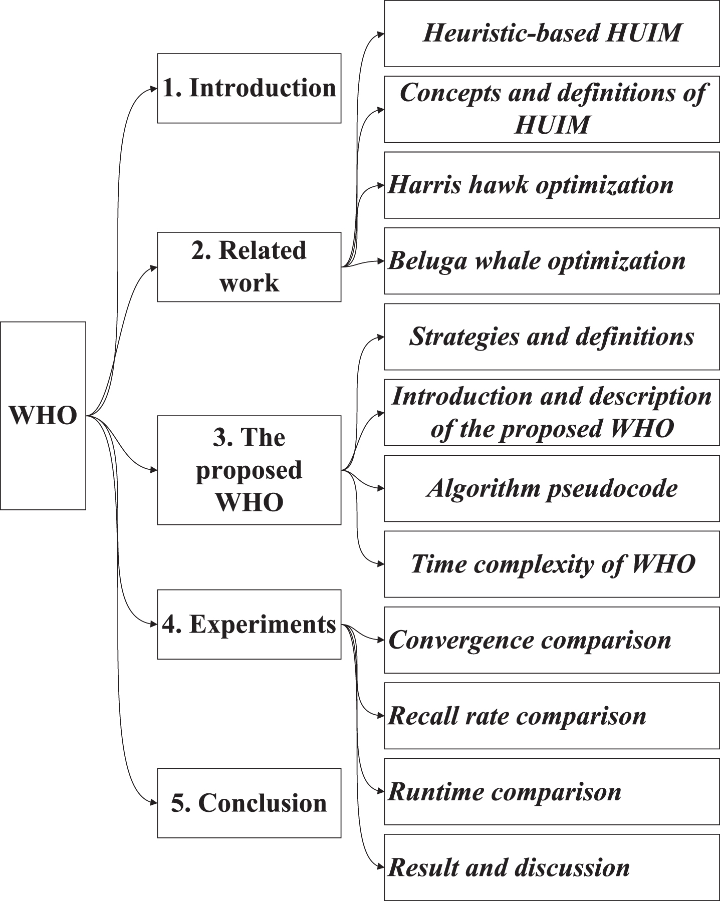
Research roadmap.

2 Related work

This chapter begins by providing an overview of heuristic high utility itemset mining methods. Then, giving the fundamental concepts of HUIM. Subsequently, the harris hawk optimization algorithm and the beluga whale optimization algorithm are introduced separately.

2.1 Heuristic-based HUIM

The application of intelligent optimization algorithms improves the efficiency of itemset mining in massive data. Previously proposed heuristic HUIM methods can be categorized into genetic algorithm (GA)-based, swarm intelligence-based, and other intelligence-based methods.

Kannimuthu et al. [11] proposed the first heuristic-based method HUPE_UMU-GRAM for mining high utility itemsets. Modeling the HUIM problem using the genetic algorithm, where genes correspond to items in the dataset, and chromosomes correspond to possible itemset combinations. The length of a chromosome is determined by the number of high transaction-weighted utility 1-itemsets in the dataset, and the fitness function value is determined by the utility of the itemset represented by the current chromosome. In addition, the mutation probability is adaptively varied according to the number of iterations and the magnitude of the fitness function value for the offspring. Based on this, Kannimuthu also proposes a top-k HUIM mining method, HUPE_WUMU-GARM, that does not require the specification of a minimum utility threshold (minutil). Song et al. [20] introduced a bio-inspired computation-based framework, Bio-HUIF, for mining HUIs. This framework utilizes bitmap encoding for itemsets and databases, where the length of the bitmap corresponds to the number of “1s” in an individual, effectively reducing memory usage. They also proposed and designed the PEVC pruning strategy to check if the itemset corresponding to the current individual exists in the original dataset. Building upon Bio-HUIF, Song et al. [20] introduced a HUIM method called Bio-HUIF-GA based on genetic algorithms. This method employs boolean changes between different positions in the vector to simulate the crossover and mutation processes typical of genetic algorithms. Zhang et al. [21] introduced a HUIM method called HUIM-IGA, based on an improved genetic algorithm. They designed a population diversity maintenance strategy that can reduce the loss of itemsets. Furthermore, a neighborhood exploration strategy for repeated HUIs was proposed to speed up the search for new HUIs. J.C.-W. Lin et al. [17] proposed the decomposition based on a compact genetic algorithm methods DcGA to mine CHUIs efficiently. This method process starts by transforming the transaction database into a graph network, an edge is created among two transactions if it exists shared item between these transactions. The community detection is applied to create a community of transactions, and each community contains highly correlated transactions. After that, the compact genetic algorithm is applied to each community for handling the grouped transactions to find the local closed high utility patterns of each community. Based on this, J.C.-W. Lin et al. proposed the multi-objective model MCUI-Miner [22] for mining the closed high utility itemsets, which employs MapReduce frameworks of a Spark structure. Experimental results demonstrate that, the MCUI-Miner outperforms the conventional CLS-Miner [23] in terms of runtime, memory use, and scalability. Luna et al. [19] proposed a top-k high utility itemsets mining method, TKHUIM-GA, based on a genetic algorithm. It guides the search process by considering the utility of each item to produce initial solutions and to combine solutions accordingly, reducing the runtime and memory consumption as a result. The proposed vertical data representation creates a list of indices of transactions in which each item appears. The length of each list denotes the support of such an item.

Swarm intelligence-based HUIM methods can be further divided into particle swarm optimization (PSO)-based, ant colony optimization (ACO)-based, and other swarm intelligence optimization-based techniques.

Particle swarm optimization algorithms, known for their simplicity, few parameters, and ease of understanding and implementation, are widely applied in high utility itemset mining. J.C.-W. Lin et al. [24] introduced a HUIM method called HUIM-BPSO_sig based on PSO. This marks the first application of PSO in HUIM. The method uses TWU pruning for initial database processing and leverages the sigmoid function to convert continuous individuals into Boolean types for individual-itemset correspondence. Based on this, J.C.-W. Lin et al. [12] introduced the HUIM-BPSO method. The proposed OR/NOR-tree structure can effectively avoid the combination of invalid particles. Based on the Bio-HUIF framework, Song et al. [20] proposed the high utility itemset mining method, Bio-HUIF-PSO, which is based on the particle swarm optimization algorithm. Initially, 1-itemset’s transaction-weighted utility (twu) is calculated, and items with twu values lower than the minutil are removed from the dataset to create a reorganized dataset. Subsequently, the bit-difference operator is utilized for population replacement and the discovery of HUIs. Wang et al. [25] introduced the HUIM-IPSO method for mining HUIs. The algorithm employs a roulette wheel selection method to probabilistically choose initial optimization values for the next generation population from the high utility itemsets of the current generation. Positions with higher TWU have a higher probability of being selected, which accelerates the mining speed of HUIs. Song et al. [26] proposed an HUIM algorithm based on set-based PSO (S-PSO) called HUIM-SPSO, and proposed the measure of the bit edit distance to reflect the diversity of the mining results. Fang et al. [27] proposed a HUIM method HUIM-IBPSO based on the improved binary particle swarm optimization. HUIM-IBPSO have multiple adjustment strategies in order to improve the mining efficiency, such as particle movement direction adjustment strategy, local exploration strategy for duplicate HUIs, restart strategy, particle modify strategy, and fitness value hash strategy. Subramaniana et al. [28] proposed GA-PSO to mine high utility itemsets. In the work, PSO is combined with GA to improve the standard PSO performance. Logeswaran et al. [29] proposed the Adaptive particle swarm optimization using reinforcement learning with off policy (APSO-RL_OFF), which employs the reinforcement learning (RL) concept to achieve the adaptive online calibration of PSO control and, in turn, to increase the performance of PSO. Gunawan et al. [30] proposed a method to improve the state-of-the-art BPSO-based high utility itemset mining by tuning the method’s initial population, inertia weight, acceleration coefficient, and velocity clamping. Yang et al. [31] proposed a particle filter-based method PF-HUIM to mine high utility itemsets. This approach first initializes a population, which consists of particle sets. Then, to update the particle sets and their weights, a novel state transition model is suggested. Finally, the approach alleviates the particle degradation problem by resampling. Sukanya et al. [32] proposed a differential evolution (DE) and (PSO)-based HUIM method HUIM-DE-PSO-DE. It using multiple strategies to discover HUIs, including elitism, population diversifications, exclusive preservations, and neighborhood exploration techniques. Song et al. [16] introduced two algorithms for mining high average utility itemsets (HAUIs): HAUI-PSO, based on the standard PSO algorithm, and HAUI-PSOD, based on the bio-inspired HUI framework Bio-HUIF. The algorithms use an initial pruning based on the average-utility upper bound (AUUB), effectively improving the algorithm’s runtime efficiency. Experimental results demonstrate that the former is more efficient, while the latter exhibits stronger convergence. Gunawan et al. [33] introduced a method, HUIM-BPSO-nomut, for mining top-k HUIs without the need for pre-setting the minutil. In the preprocessing stage, the algorithm sorts the original dataset based on the transaction utility, and it employs binary particle swarm optimization (BPSO) to mine itemsets. The discovered itemsets are then output in order of utility value in a list, with the minutil added to the list for subsequent processing steps.

Ant colony algorithm is a bio-inspired algorithm derived from the natural world, which extensively draws from the foraging behavior of ants. Wu et al. [34] introduced a high utility itemset mining method based on ant colony algorithm, named HUIM-ACS. This method maps the complete solution space of the HUIM problem into a routing graph. It includes two pruning processes, positive pruning and recursive pruning, to avoid unnecessary estimations of itemsets. Additionally, it introduces a checking mechanism to verify the discovery of all HUIs in the dataset. Infrequent itemsets are rare but may yield significant returns. Arunkumar et al. [35] introduced a method called ACHUIIM, which uses the ant colony algorithm to mine infrequent high utility itemsets (IHUIs). If an itemset is high utility and has no superset with the same support, it is referred to as a closed high utility itemset (CHUIs). Pramanik et al. [36] introduced a method called CHUI-AC, based on the ant colony algorithm, which modified the global update rules and the improved routing graph with l + 1 nodes, resulting in l(l + 1)/2 edges.

Other swarm intelligence optimization algorithms like artificial bee colony (ABC), bat algorithm (BA), grey wolf optimization algorithm (BWO), artificial fish swarm algorithm (AFSA), and more, can also be applied to high utility itemset mining. HUIM-ABC method was proposed by Song et al. [13] which models HUIM from the perspective of the ABC. The original dataset is converted into a bitmap format, and a promising bit vector check (PBVC) pruning strategy is designed to trim the search space and accelerate algorithm convergence. Additionally, the direct nectar source generation (DNSG) strategy was proposed to generate more promising new nectar sources as early as possible so that more HUIs can be discovered within a certain number of cycles and the computational cost can also be lowered. Based on the Bio-HUIF framework, Song et al. [20] introduced the high utility itemset mining method, Bio-HUIF-BA, based on the bat algorithm. They rewrote the bat’s position update formula and used boolean operations on bitmap bit vectors to simulate the bat’s exploration process. Pazhaniraja et al. [37] introduced the binary grey wolf optimization algorithm (BGWO) and applied it to HUIM, proposing the BGWO-HUI method. The proposed model is modelled with Boolean operations such as De Morgans’s AND, Adder, Difference, Circular Shift and Multiplexer. Pazhaniraja et al. [38] proposed a high utility itemsets mining methods HUIM-DE which is based on GA and the dolphin echolocation optimization (DEO). The algorithm has two variants: one that utilizes a minimum utility threshold to mine all HUIs in the dataset, and another that doesn’t use a minimum utility threshold to mine the top-k HUIs. Building upon BGWO-HUI and HUIM-DEO, Pazhaniraja et al. [11] introduced a new heuristic algorithm, DE-BGWO, which combines dolphin echolocation (DE) and binary grey wolf optimization algorithms (BGWO). This hybrid algorithm was then applied to the problem of HUIM. Song et al. [14] proposed the HUIM-AF method, model the HUI mining problem with three behaviors of artificial fish: follow, swarm, and prey.

Apart from the algorithms mentioned above, other intelligent optimization algorithms like differential evolution (DE), multi-objective evolutionary algorithm (MOEA), cross-entropy (CE), and more have also been applied to the mining of HUIs. Differential evolution has long been successfully applied to solving the problems of high dimensions. Further DE is robust and quick compared to GA. Therefore, Krishna et al. [39] proposed TNR-HUARM methods to mine top non-redundant high utility association rule, the method is based on binary differential evolution (BDE) and an adaptive binary differential evolution (ABDE). Furthermore, the author explored a possible application of the TNR-HUARM for the analytical CRM, i.e. customer segmentation based on monetary value of the customers. Unlike HUIM, in the TNR-HUARM method, fitness is defined as the product of utility value and confidence. Based on this, Krishna et al. [40] introduced a HUIM method based on DE. This method has two different variants, namely HUIM-BDE, which is based on binary differential evolution, and HUIM-ABDE, which is based on adaptive binary differential evolution. Usually, the higher support of an itemset X will lead to lower utility in most cases, while the lower support of X often leads to higher utility. Zhang et al. [41] considered support and utility in a unified framework from a multi-objective view, transformed the problem of mining frequent and high utility itemsets (FHUIs) as a 2-objective problem. They proposed a multi-objective evolutionary algorithm named MOEA-FHUI to solve the transformed multi-objective itemset mining, which does not need to specify the prior parameters such minimal support threshold and minimal utility threshold. Cao et al. [42] introduced two update strategies, including updating strategy based on closed itemsets (USC) and updating strategy based on approximate-closed itemsets (USA)£¬with the aim of accelerating the convergence of population as well as improving the diversity of population. Based on these two strategies, an effective multi-objective evolutionary algorithm, names CP-MOEA, is suggested for the task of mining FHUIs. The CP-MOEA adopts the similar framework with NSGA-II [43], where two objectives, namely support and utility, are optimized simultaneously. When both the number of transactions and the number of items in a transaction database are large, MOEA may be inefficient. To address this issue, Fang et al. [44] proposed BOEA-FHUI for mining FHUIs based on the bio-objective evolutionary algorithm (BOEA). This method includes three strategies, namely TWU pruning strategy, repair strategy, and the improved mutation strategy. Ahmed et al. [45] considered both utility and uncertainty as the majority objects, developed a multi-objective evolutionary approach MOEA-HEUPM to mine high expected utility patterns (HEUPs) model. Two encoding schemas, binary encoding and value encoding are developed and utilized in the designed MOEA-HEUPM model. In most cases, the higher the support of a pattern, the lower the occupancy and utility value, and the lower the support of the pattern, the higher the occupancy and utility value. In order to get the maximum compromise solution, Fang et al. [46] proposed a multi-objective problem model MOEA-PM to mine high quality patterns (HQPs), where the objectives are support, occupancy, and utility. Two kinds of population initialization strategies are designed, which is used to ensure the population is effectively distributed in the feasible solution space. Song et al. [18] proposed two algorithms, called the top-k high utility itemset mining based on cross-entropy method (TKU-CE) and TKU-CE+, for mining the top-k HUIs heuristically. The TKU-CE algorithm is based on cross-entropy, and implements top-k HUI mining using combinatorial optimization. The main idea of TKU-CE is to generate the top-k HUIs by gradually updating the probabilities of itemsets with high-utility values. TKU-CE+ optimizes TKU-CE in three respects. First, unpromising items are filtered by critical utility value, to reduce the computational burden in the initial stage. Second, a sample refinement strategy is used in each iteration, to reduce the computational burden in the iterative stage. Finally, smoothing mutation is proposed, to randomly generate some new itemsets in addition to those from previous iterations. Consequently, diversity of samples is improved, so that more actual top-k HUIs can be discovered with fewer iterations. Nawaz et al. [6] modeled the problem of HUIM from the perspective of HC and SA algorithms. The database is converted into a bitmap, which is used both for information representation and search space pruning. Instead of maintaining the HUIs with highest utility value from population to population, the strategy of selecting discovered HUIs probabilistically for the next population is used. This strategy allows to discover more HUIs in less iteration cycles.

Table 3 provides a summary of heuristic-based HUIM methods, categorizing and ranking them based on the related publications, research objectives, and applications. In the table, “n” represents the population size, “T” represents the algorithm’s maximum number of iterations, and “d” represents the length of individuals.

Table 1
Utility list

item A B C D E F

external utility 1 3 2 4 1 2

item	A	B	C	D	E	F
external utility	1	3	2	4	1	2

Table 2

Transaction list

tid	transactions	tu
T ₁	(A, 4) (B, 4) (D, 3)	28
T ₂	(B, 3) (C, 4) (D, 1) (E, 2)	23
T ₃	(A, 2) (B, 1) (C, 3) (D, 3) (F, 2)	27
T ₄	(B, 3) (C, 4) (E, 4) (F, 1)	23

Table 3

Summary of heuristic-based high utility itemset mining methods

Algorithm	Year	Authors	Publication	Objectives	Applications	Pruning strategy	Update strategy	Comparison algorithms	Datasets	Parameter	Advantages	Disadvantages
MOEA-HEUPM [45]	2020	Ahmed et al.	IEEE transactions on emerging topics in computational intelligence	MOEA	HEUPs	None	meta-itemset-selection, transaction-itemset-selection	U-Apriori, EFIM	chess, mushroom, accidents, retail, pumsb, kosarak, T10I4N4KDXK	n = 100, T = 100	Can discover the valuable HEUPs without pre-defined threshold values in the uncertain environment.	Tends to miss patterns.
CP-MOEA [42]	2019	Cao et al.	2019 IEEE congress on evolutionary computation	MOEA	FHUIs	None	USC, USA, NSGA-II-based	MOEA-FHUI	chess, connect_50%, mushroom, accidents_10%, USCensus_10%, Pamp_10%	n = 100, T = 200	The proposed strategies, USC and USA, can enhance population diversity and accelerate convergence. It outperforms the MOEA-FHUI algorithm in terms of convergence and Hypervolume (HV).	No experiments on large datasets.
HUIM-HC [6]	2021	Nawaz et al.	ACM Transactions on Management Information System	HC	HUIs	TWU	bitmap-based, roulette wheel selection	HUIF-GA, HUIF-PSO, HUIF-BA, HUPE_UMU-GRAM, HUIM-BPSO_sig, HUIM-BPSO	chess, connect, mushroom, accidents_10%, foodmart, Ecommerce	n = 30, T = 10000, d = \|1-HTWUI\|	High efficient; the runtime is relatively insensitive to the minutil; low memory usage	Easily trapped into local optimal, potentially leading to the loss of itemsets; poor convergence.
Algorithm	Year	Authors	Publication	Objectives	Applications	Pruning strategy	Update strategy	Comparison algorithms	Datasets	Parameter	Advantages	Disadvantages
HUIM-SA [6]	2021	Nawaz et al.	ACM Transactions on Management Information System	SA	HUIs	TWU	bitmap-based, roulette wheel selection	HUIF-GA, HUIF-PSO, HUIF-BA, HUPE_UMU-GRAM, HUIM-BPSO_sig, HUIM-BPSO	chess, connect, mushroom, accidents_10%, foodmart, Ecommerce	T = 10000, d = \|1-HTWUI\|	High efficiency.	Consumes large amount of memory; easily misses itemsets; poor convergence
HUIM-SPSO [26]	2020	Song et al.	Advanced Data Mining and Applications: 16th International Conference, ADMA 2020	PSO	HUIs	TWU	set-based, roulette wheel selection, bitmap-based	HUIM-BPSO_sig, HUIM-BPSO	chess, connect, mushroom, accidents_10%	n = 20, T = 10000, d = \|1-HTWUI\|	The algorithm exhibits stable runtime and less affected by the minutil.	Tends to miss itemsets; poor performance on sparse datasets.
HUIM-ABC [13]	2018	Song et al.	Advances in Knowledge Discovery and Data Mining: 22nd Pacific-Asia Conference, PAKDD 2018	ABC	HUIs	TWU, PBVC	bitmap-based	HUPE_UMU-GRAM, HUIM-BPSO_sig, HUIM-BPSO	chess, connect, mushroom, accidents_10%	T = 10000	The useless operation of utility calculation could be avoided, the HUIM-ABC outperformed HUPE_UMU-GARM, HUIM-BPSO_sig, HUIM-BPSO in runtime, number of discovered HUIs and convergence.	Tends to miss itemsets; poor performance on sparse datasets.
HUIM-AF [14]	2021	Song et al.	Advances in Swarm Intelligence: 12th International Conference, ICSI 2021	AFSA	HUIs	TWU	bitmap-based, roulette wheel selection	HUPE_UMU-GRAM, HUIM-BPSO_sig	chess, connect, mushroom, accidents_10%	n = 20, T = 10000, d = \|1-HTWUI\|	Performs efficiently in dense datasets	Not suitable* for sparse datasets.
HUPE_UMU-GRAM [11]	2014	Kannimuthu et al.	Applied Artificial Intelligence	GA	HUIs	TWU	roulette wheel selection	None	T10I4D10K	T = 100, d = \|1-HTWUI\|	This is the first heuristic-based algorithm for high utility itemsets mining.	Poor convergence and a large number of itemsets are missed.
CHUI-AC [36]	2021	Pramanik et al.	Applied Intelligence	ACS	CHUIs	TWU	modified ant routing graph-based	HUIM-ACS, CHUD, CHUI-Miner, Bio-HUIF-PSO, Bio-HUIF-GA, HUIM-BPSO	chess, mushroom, foodmart, retail, BMS, chainstore	n = 100, T = 10000, d = \|1-HTWUI\|	Good convergence and scalability.	Poor performance on highly sparse datasets.
TKU-CE+ [18]	2021	Song et al.	Applied Intelligence	CE	top-k HUIs	TWU, critical utility value-based	bitmap-based	TKU, TKO, kHMC	chess, chainstore, pumsb, T35I100D7k, T50I150D10k, T40I100D20k	n = 2000, T = 2000, d = \|I\|	Good scalability, high efficiency, and low memory usage.	Slower convergence speed and may miss some genuine top-k HUIs.
MOEA-FHUI [41]	2018	Zhang et al.	Applied Soft Computing	MOEA	FHUIs	None	support-based, MOEA/D-based	FP-Growth, HUI-Miner, HUIM-ACS, TKU-Miner	chess, connect_50%, mushroom, accidents_10%, foodmart, OnlineRetail_10%, USCensus_10%, Pamp_10%, Kddcup99_10%, Susy_1%, BMS-Web-View-1, Powerc_10%	n = 100, T = 300	The high utility itemsets mined are frequent; does not need to specify the prior parameters such as minimal support threshold and minimal utility threshold.	The solution lacks diversity and has poor convergence, leading to the miss of itemsets. It is difficult to obtain the itemsets for a specified threshold.
HUIM-IBPSO [27]	2022	Fang et al.	Applied Soft Computing	PSO	HUIs	TWU	bitmap-based, roulette wheel selection, sigmoid function-based	HUIM-BPSO_sig, HUIM-BPSO, Bio-HUIF-PSO, Bio-HUIF-GA, HUPE_UMU-GRAM	chess, mushroom, connect, accidents_10%	n = 20, T = 3000, d = \|1-HTWUI\|	High convergence; lower number of missing itemsets; high efficiency	Tends to miss itemsets; no experiments on large datasets.
BOEA-FHUI [44]	2023	Fang et al.	Applied Soft Computing	BOEA	FHUIs	TWU	NSGA-II-based	MOEA-PM, MOEA-FHUI, SparseEA	chess, connect, mushroom, accidents_10%, PAMAP_10%, USCensus_10%, pumsb, C73d10k	n = 50, T = 10000, d = \|I\|	Good convergence.	Tends to miss patterns.
DcGA [17]	2021	J.C.-W. Lin et al.	Applied Soft Computing Journal	GA	CHUIs	community detection	vector of probability-based	CLS-Miner, CHUI-Miner	SIGN, Leviathan, MSNBC, BMS	T = 100	Ability to mine the concise itemsets. The community detection ensures that more complete CHUIs would be discovered.	Some itemsets will be missed.
HAUI-PSO [16]	2020	Song et al.	Data Science and Pattern Recognition	PSO	HAUI	AUUB	roulette wheel selection	HAUI-Miner, EHAUPM	chess, connect, accidents_10% T25N100D50K	n = 20, T = 1000	The runtime is relatively insensitive to the minutil.	Poor convergence; missing a large number of itemsets.
HAUI-PSOD [16]	2020	Song et al.	Data Science and Pattern Recognition	PSO	HAUI	AUUB	roulette wheel selection	HAUI-Miner, EHAUPM	chess, connect, accidents_10% T25N100D50K	n = 20, T = 1000	The runtime is relatively insensitive to the minutil.	The runtime is longer when dealing with datasets containing a larger number of items. Tends to miss itemsets.
HUIM-BPSO_sig [24]	2016	J.C.-W. Lin et al.	Engineering Applications of Artificial Intelligence	PSO	HUIs	TWU	sigmoid function-based	HUPE_UMU-GRAM, HUI-Miner	chess, connect, mushroom, accidents_10%	n = 20, T = 10000, d = \|1-HTWUI\|	Fewer parameters are used than genetic algorithms.	Tends to miss itemsets; poor performance on sparse datasets.
TNR-HUARM [39]	2020	Krishna et al.	Engineering Applications of Artificial Intelligence	DE	top high utility association rules	None	sigmoid function-based	LNR-HAR, HGB*	chess, connect, mushroom, accidents_10%, foodmart, retail, OnlineRetail	n = 20, T = 10000	Fared well in terms ofexecution time, memory and convergence.	Some patterns will be missed.
HUIM-ABDE [40]	2021	Krishna et al.	Expert Systems With Applications	DE	HUIs	None	sigmoid function-based	HUIM-BPSO_sig, HUI-BPSO, HUPE_UMU-GRAM, HUI-ACS, HUIM-BPSO-nomut	chess, connect, mushroom, accidents_10%, foodmart, retail, OnlineRetail	n = 20, T = 10000, d = \|I\|	No need for manual adjustment of control parameters due to the adaptive binary differential evolution method.	Tends to miss itemsets.
Bio-HUIF-BA [20]	2018	Song et al.	IEEE Access	BA	HUIs	TWU, PEVC	bitmap-based, roulette wheel selection	HUPE_UMU-GRAM, HUIM-BPSO, IHUP, UP-Growth	chess, connect, mushroom, accidents_10%	n = 20, T = 2000, d = \|1-HTWUI\|	Utilizing bitmap encoding for individuals can effectively reduce memory usage.	Easily misses itemsets; no experiments were performed on sparse datasets.
Bio-HUIF-GA [20]	2018	Song et al.	IEEE Access	GA	HUIs	TWU, PEVC	bitmap-based, roulette wheel selection	HUPE_UMU-GRAM, HUIM-BPSO, IHUP, UP-Growth	chess, connect, mushroom, accidents_10%	n = 20, T = 2000, d = \|1-HTWUI\|	Utilizing bitmap encoding for individuals can effectively reduce memory usage.	Easily misses itemsets; no experiments were performed on sparse datasets.
Bio-HUIF-PSO [20]	2018	Song et al.	IEEE Access	PSO	HUIs	TWU, PEVC	bitmap-based, roulette wheel selection	HUPE_UMU-GRAM, HUIM-BPSO, IHUP, UP-Growth	chess, connect, mushroom, accidents_10%	n = 20, T = 2000, d = \|1-HTWUI\|	Utilizing bitmaps to encode individuals can effectively reduce the memory usage.	Easily misses itemsets; no experiments on sparse datasets.
HUIM-IGA [21]	2019	Zhang et al.	IEEE Access	GA	HUIs	TWU	bitmap-based, roulette wheel selection	Bio-HUIF-GA, Bio-HUIF-PSO, HUIM-BPSO, HUIM-BPSO_sig, HUPE_UMU-GRAM, IHUP, UP-Growth, UP-Hist Growth	chess, connect, mushroom, accidents_10%	n = 20, T = 3000, d = \|1-HTWUI\|	Runs efficiently and exhibits good convergence.	Tends to miss itemsets.
MOEA-PM [46]	2020	Fang et al.	IEEE Transactions on Knowledge and Data Engineering	MOEA	HQPs	None	NSGA-II-based, bitmap-based,	MOEA-FHUI	chess, connect, mushroom, accident_10%, PAMAP_10%, USCensus_10%	n = 50, T = 10000, d = \|I\|	Can discover patterns that are both frequently occurring and has a high utility in the transaction datasets, while at the same time being relatively complete.	Tends to miss patterns.
TKHUIM-GA [19]	2023	Luna et al.	Information Sciences	GA	top-k HUIs	None	indices list-based	HUPE_UMU-GRAM, HUIM-BPSO_sig, HUIM-BPSO, Bio-HUIF-PSO, Bio-HUIF-GA, Bio-HUIF-BA, HUIM-ABC, HUIM-SPSO, HUIM-AF, HUIM-HC, HUIM-SA, TKU, TKO	chess, ChessNeg, foodmart, mushroom, MushroomNeg, Liquor, Ecommerce, pumsb, BMS, connect, retail, RetailNeg, Fruithut, accidents, AccidentsNeg, kosarak, KosarakNeg, chainStore	n = 50	Works on positive, negative, integer and real unit utility values	Uncertainty about whether the optimal solution can be found; the uncertainty that the best solutions are found.
APSO-RL_OFF [29]	2023	Logeswaran et al.	Information Technology and Control	PSO	HUIs	TWU	sigmoid function-based	HUPE_UMU-GRAM, HUIM-BPSO	chess, connect, mushroom, accidents_10%	n = 30, T = 2500, d = \|1-HTWUI\|	Efficient.	Easily misses itemset; no experiments on sparse datasets
HUIM-DE-PSO-DE [32]	2023	Sukanya et al.	International Journal of Computational Intelligence and Applications	DE, PSO	HUIs	TWU	elitism technique	DEO, HUIM-IGA, Bio-HUIF-PSO, greedy search	chess, connect, mushroom, accidents_10%	n = 99, T = 1000, d = \|1-HTWUI\|	High efficiency.	Tends to miss itemsets; no experiments on sparse datasets.
ACHUIIM [35]	2018	Arunkumar et al.	International Journal of Parallel Programming	ACS	HUIIs	utility-based	routing graph-based	HURI	chess, mushroom, retail, foodmart	n = 40, 50, 60	Shorter run time.	Runtime is strongly influenced by the minutil.
HUIM-DEO [38]	2021	Pazhaniraja et al.	Journal of Ambient Intelligence and Humanized Computing	GA, DEO	HUIs; top-k HUIs	TWU	roulette wheel selection	HUPE_UMU-GRAM, Bio-HUIF-GA, HUIM-BPSO, Bio-HUIF-PSO	chess, connect, mushroom, accidents_8%	T = 800, d = \|1-HTWUI\|	Shorter run time.	Tends to miss itemsets; no experiments on sparse datasets.
DE-BGWO [15]	2023	Pazhaniraja et al.	Journal of Ambient Intelligence and Humanized Computing	DE-BGWO	HUIs	TWU	bitmap-based, roulette wheel selection	Greedy search-based, GA-based, BGWO-based, DEO-based	chess, connect, mushroom, accidents_8%	T = 800, d = \|1-HTWUI\|	The runtime is relatively insensitive to the minutil.	Easily misses itemset.
HUIM-IPSO [25]	2020	Wang et al.	Journal of Chinese Computer Systems	PSO	HUIs	TWU, PEVC	bitmap-based, roulette wheel selection	HUIM-BPSO, HUPE_UMU-GRAM	chess, mushroom, foodmart, retail	n = 30, T = 1000, d = \|1-HTWUI\|	The roulette wheel selection method tends to enhance the exploration efficiency of the algorithm in its early stages and exhibits favorable convergence properties.	Easily trapped into local optimal, potentially leading to the loss of itemsets; no experiments on large datasets.
HUIM-ACS [34]	2016	Wu et al.	Knowledge-Based Systems	ACS	HUIs	TWU, positive pruning, recursive pruning	routing graph-based	HUPE_UMU-GRAM, EFIM, HUIM-BPSO, HUI-Miner	chess, connect, mushroom, accidents_10%, foodmart, retail	n = 20, T = 10000, d = \|1-HTWUI\|	Shorter run time, higher number of itemsets that can be mined.	Rely on pruning rules and prioritizes the search for itemsets with high transaction-weighted utility, which can result in the loss of many itemsets with lower transaction-weighted utility. Requires a lot of memory to store the route map.
HUIM-IPSO [25]	2020	Wang et al.	Journal of Chinese Computer Systems	PSO	HUIs	TWU, PEVC	bitmap-based, roulette wheel selection	HUIM-BPSO, HUPE_UMU-GRAM	chess, mushroom, foodmart, retail	n = 30, T = 1000, d = \|1-HTWUI\|	The roulette wheel selection method tends to enhance the exploration efficiency of the algorithm in its early stages and exhibits favorable convergence properties.	Easily trapped into local optimal, potentially leading to the loss of itemsets; no experiments on large datasets.
HUIM-ACS [34]	2016	Wu et al.	Knowledge-Based Systems	ACS	HUIs	TWU, positive pruning, recursive pruning	routing graph-based	HUPE_UMU-GRAM, EFIM, HUIM-BPSO, HUI-Miner	chess, connect, mushroom, accidents_10%, foodmart, retail	n = 20, T = 10000, d = \|1-HTWUI\|	Shorter run time, higher number of itemsets that can be mined.	Rely on pruning rules and prioritizes the search for itemsets with high transaction-weighted utility, which can result in the loss of many itemsets with lower transaction-weighted utility. Requires a lot of memory to store the route map.
HUIM-BPSO-nomut [33]	2020	Gunawan et al.	Knowledge-Based Systems	PSO	top-k HUIs	None	roulette wheel selection, sigmoid function-based	TKU, TKO, kHMC, HUPE_UMU-GRAM£¬HUIM-BPSO, HUIM-ACS, Bio-HUIF-GA, Bio-HUIF-PSO, Bio-HUIF-BA	chess, connect, mushroom, accidents_10%, foodmart	n = 20, T = 10000	No need to pre-set the minutil.	Poor performance on sparse datasets.
PF-HUIM [31]	2023	Yang et al.	Mathematical Problems in Engineering	PSO	HUIs	TWU	bitmap-based	HUPEumu-GRAM, Bio-HUIF-PSO, HUIM-BPSO	chess, connect, mushroom, foodmart, BMS, Crimes in, Chicago	T = 1000, d = \|1-HTWUI\|	High efficiency.	Tends to miss itemsets.
HUIM-BPSO [12]	2016	J.C.-W. Lin et al.	Soft Compute	PSO	HUIs	TWU, OR/NOR-tree	sigmoid function-based	HUPE_UMU-GRAM	chess, connect, mushroom, accidents_10%, foodmart, retail	n = 20, T = 10000, d = \|1-HTWUI\|	Fewer parameters are used than genetic algorithms; the proposed OR/NOR-tree structure can effectively avoid invalid particle combinations.	Tends to miss itemsets; poor performance on sparse datasets.
BGWO-HUI [37]	2020	Pazhaniraja et al.	Soft Computing	BGWO	HUIs	TWU	boolean operations-based	HUPE_UMU-GRAM, HUIM-BPSO, IHUP, UP-Growth, Bio-HUIF-GA, Bio-HUIF-PSO, Bio-HUIF-BA	chess, connect, mushroom, accidents	n = 100, T = 2000, d = \|1-HTWUI\|	Fewer parameters and higher recall.	Tends to miss itemsets; no experiments on sparse datasets.

2.2 Concepts and definitions of HUIM

This section introduces the HUIM and the related definition of HUIM in data streams. Let I = {i₁, i₂, i₃,..., i_n} be a set of items, and let DB be a database with a utility list (Table 1) and a transaction list (Table 2). In Table 2, each row represents a transaction, where each letter within the transaction denotes an item along with its corresponding internal utility displayed on the right-hand side. Within the transaction list, each transaction denoted as T, possesses a unique identifier which is expressed as tid. A set of items is referred to as a k-itemset if it is a subset of I and consists of k elements.

Definition 1 (external utility) [2]. The external utility of item i is symbolized as eu(i), which corresponds to the utility value of i in the utility table.

For instance, considering Table 1, item “A” has an external utility denoted as eu(A) equal to 1.

Definition 2 (internal utility) [2]. The internal utility of item i within transaction T is represented as iu(i, T), which signifies the numerical value assigned to i in T within the transaction list.

For instance, considering Table 2, the internal utility of item “A” within T₁ is denoted as iu(A, T₁) and has a value of 4.

Definition 3 (utility of item in transaction) [3]. The utility of i in T, represented as u(i, T), is determined by the product of its internal utility and external utility, as expressed in Equation (1). $u (i, T) = iu (i, T) \times eu (i)$ (1)

According to the given example, when considering the utility of item “A” in T₁, the calculation is performed as follows: u(A, T₁) = iu(A, T₁)×eu(A) = 4×1 = 4. This demonstrates that the utility of “A” in T₁ is determined to be 4.

Definition 4 (utility of itemset in transaction) [3]. Assuming that X is an itemset, the utility of X in T denoted as u(X, T), is obtained by summing the utilities of all items in X. It should be noted that X represents a set of items and is considered as a subset of transaction This can be expressed mathematically using Equation (2). $u (X, T) = \sum_{i \in X \land X \subseteq T} u (i, T)$ (2)

For instance, let’s examine the utility of the itemset {A, B} in two different transactions, T₁ and T₃. In transaction T₁, we calculate the utility of {A, B} by summing the utilities of items a and b within T₁. Thus, u({A, B}, T₁) is determined as u(A, T₁)+u(B, T₁), which evaluates to 4×1 + 4×3 = 16. Similarly, in transaction T₃, the utility of {a, b} is computed by adding the utilities of items a and b within T₃. Hence, u({A, B}, T₃) equals u(A, T₃) + u(B, T₃), resulting in 2×1 + 1×3 = 5.

Definition 5 (utility of itemset) [4]. The utility of an itemset X, represented by u(X), is obtained by summing the utilities of the itemset X across all transactions T that contain X in DB. This relationship is expressed mathematically using Equation (3). $u (X) = \sum_{T \in DB \land X \subseteq T} u (X, T)$ (3)

For instance, the utility of the {A, B} denoted as u({A, B}), is obtained as the sum of u({A, B}, T₁) and u({A, B}, T₃), resulting in a value of 16 + 5 = 21.

Definition 6 (high utility itemset) [3]. An itemset X is considered a high utility itemset, abbreviated as HUI, if its utility is not less than the minutil.

Definition 7 (high utility itemset mining) [3]. The task of high utility itemset mining is to discover all high utility itemsets within a database.

Definition 8 (utility of a transaction) [4]. The utility of a transaction T, represented by tu(T), is calculated by summing the utilities of all items within T. The total utility of the database DB is obtained by summing the utilities of all transactions within DB. This relationship is defined by Equation (4). $tu (T) = \sum_{i \in T} u (i, T)$ (4)

The cumulative utility of the database in Table 1 is obtained by summing the individual utilities of all transactions. It can be expressed as the sum of tu(T₁), tu(T₂), tu(T₃), tu(T₄), tu(T₅), and tu(T₆), which evaluates to 28 + 23 + 27 + 23 + 16 + 12 = 129. This calculation reflects the total utility derived from all transactions and signifies the overall utility of the database.

Definition 9 (transaction-weighted utility of an itemset) [2]. The transaction-weighted utility of an itemset X in DB, represented as twu(X), is determined by summing the utilities of all transactions that contain the itemset X. This calculation is carried out within the context of the database DB and can be expressed using Equation (5). $twu (X) = \sum_{T \in DB \land X \subseteq T} tu (T)$ (5)

For instance, the twu of {A} can be calculated by summing the transaction utilities of all transactions containing the itemset in the database and is obtained as the sum of tu(T₁), tu(T₃), and tu(T₅) which equal 28, 27, and 16, respectively, resulting in a total twu of 71. The twu values for all 1-itemsets in the database are presented in Table 4, showcasing the contributions of these itemsets to the overall utility of the transactions.

Table 4

The twu of 1-itemsets

Itemset	{A}	{B}	{C}	{D}	{E}	{F}
Twu	55	101	73	78	46	50

Definition 10 (high transaction-weighted utility itemset) [18]. An itemset X is a high transaction-weighted utility itemset (HTWUI) if the twu of the itemset X is not less than minutil in DB.

Definition 11 (low transaction-weighted utility itemset) [18]. An itemset X is a low transaction-weighted utility itemset (LTWUI) if the transaction-weighted utility of the itemset X is less than minutil in DB.

For example, if minutil = 70, there are five 1-HTWUIs in DB, {A}, {B}, {C}, {D}, {E}, and the 1-LTWUI is {F}, because only {F} has a twu less than 70, and all the other 1-itemsets have a transaction-weighted utility no less than 70.

2.3 Harris hawk optimization

Harris hawk optimization [47] is a heuristic algorithm proposed by Heidari et al. in 2019.

The HHO approach employs hawks as the representation of candidate solutions, with the optimal or nearly optimal solution being referred to as the prey. The HHO is divided into the exploration phase and exploitation phase, in the exploitation phase the hawk changes its behavior according to the escape energy of prey. The escape energy E of the prey is shown in Equation (6). Where t is the number of current iterations, T is the maximum number of iterations, E₀ is the initial escape energy of the prey (obtained from Equation (7)), and r is a random number in [0, 1]. $E = 2 E_{0} (1 - \frac{t}{T})$ (6) $E_{0} = 2 r - 1$ (7)

(1) Exploration phase

During the exploration phase, the position of the hawk is updated using Equation (8). This equation incorporates various variables, such as X, X_k, X_r, t, ub, lb, r₁, r₂, r₃, r₄, and q. Specifically, X represents the position of the hawk, X_k represents the position of a randomly chosen hawk, X_r represents the position of the prey (i.e., the global optimal solution or gbest), and ub and lb represent the upper and lower bounds of the search space. Additionally, the equation involves five random numbers (r₁, r₂, r₃, r₄, and q), each of which falls within the range [0, 1]. X_m denotes the mean position of the current population and can be calculated as shown in Equation (9). X_n refers to the nth hawk in the current population, while Num represents the total number of hawks in the population (i.e., population size) [47]. $\begin{matrix} X (t + 1) = \\ {\begin{matrix} X_{k} (t) - r_{1} | X_{k} (t) - 2 r_{2} X (t) | & q ⩾ 0.5 \\ (X_{r} (t) - X_{m} (t)) + r_{3} (lb + r_{4} (ub - lb)) & q < 0.5 \end{matrix} \end{matrix}$ (8) $X_{m} (t) = \frac{1}{Num} \sum_{n = 1}^{Num} X_{n} (t)$ (9)

(2) Exploitation phase

a. Soft besiege

During a soft besiege scenario, r is greater than or equal to 0.5 and the absolute value of E is no less than 0.5. To update the hawk’s position, Equation (10) is employed, which considers several parameters such as ΔX, J, and r₅. ΔX refers to the distance between the current hawk and its prey while J represents the jump energy, which is calculated using Equations (11) and (12). Additionally, r₅ is a random number generated within the range of [0, 1] during every iteration [47]. $X (t + 1) = Δ X (t) - E | {JX}_{r} (t) - X (t) |$ (10) $Δ X (t) = X_{r} (t) - X (t)$ (11) $J = 2 (1 - r_{5})$ (12)

b. Hard besiege

The hard besiege arise when r≥0.5 and |E| < 0.5. During such times, Equation (13) is employed to update the hawk’s location [47]. $X (t + 1) = X_{r} (t) - E | Δ X (t) |$ (13)

c. Soft besiege with progressive rapid dives

If r is less than 0.5 and the absolute value of E is greater than or equal to 0.5, a gradual dive strategy is executed, known as soft besiege with progressive rapid dives. This tactic updates the hawk’s position using Equation (14) [47]. $X (t + 1) = {\begin{matrix} Y, & if F (Y) < F (X (t)) \\ X, & if F (Z) < F (X (t)) \end{matrix}$ (14)

In the above equation, F (.) represents the fitness function, while Y and Z are the two hawks newly generated using Equations (15) and (16), respectively. The variable D denotes the dimension of the hawk, α is a random D-dimensional vector, and the function Levy (Equation (17)) represents the Levy flight [47]. $Y = X_{r} (t) - E | {JX}_{r} (t) - X (t) |$ (15) $Z = Y + α \times Levy (D)$ (16) $Levy (D) = 0.01 \times \frac{μ \times σ}{{| ν |}^{1 / - β}}$ (17)

In this equation, μ and ν are two distinct random numbers that originate from a normal distribution. σ can be computed using Equation (18), while β is a predefined constant with a value of 1.5 [47]. $σ = {(\frac{Γ (1 + β) \times sin (\frac{π β}{2})}{Γ (\frac{1 + β}{2}) \times β \times 2^{(\frac{β - 1}{2})}})}^{\frac{1}{β}}$ (18)

d. Hard besiege with progressive rapid dives

During instances where r is less than 0.5 and the absolute value of E is also less than 0.5, the HHO executes the hard besiege with progressive rapid dives. To update the hawk’s position in this scenario, Equation (19) is applied [47]. $X (t + 1) = {\begin{matrix} Y, & if F (Y) < F (X (t)) \\ X, & if F (Z) < F (X (t)) \end{matrix}$ (19)

Where F(.) is the fitness function, Y and Z are the two most recently generated hawks obtained from Equations (20) and (21) respectively [47]. $Y = X_{r} (t) - E | {JX}_{r} (t) - X_{m} (t) |$ (20) $Z = Y + α \times Levy (D)$ (21)

Too et al. [48] introduced the binary harris hawk optimization algorithm (BHHO) for feature selection. In the t-th iteration, the position of the i-th hawk in the d-th dimension is represented as X_i^d(t), and the position obtained using HHO for the (t + 1)-th iteration is denoted as ΔX_i^d(t + 1). At this point, ΔX_i^d(t + 1) is a continuous variable. BHHO converts this continuous variable into a Boolean variable using Equations (22) to (23). $X_{i}^{d} (t + 1) = {\begin{matrix} 1 & if rand () < T (Δ X_{i}^{d} (t + 1)) \\ 0 & otherwise \end{matrix}$ (22) $T (x) = \frac{1}{1 + e^{- x}}$ (23)

2.4 Beluga whale optimization

The beluga whale optimization algorithm [49] is a metaheuristic optimization algorithm introduced in 2022, drawing inspiration from the behavioral patterns of beluga whales. Beluga whales are famous for their pure white coloration as adults and are highly social animals that form groups. Much like other metaheuristic approaches, BWO comprises exploration and exploitation phases. Furthermore, this algorithm replicates the phenomenon of whale pods observed in the natural world.

In the beluga whale optimization algorithm, each beluga whale is considered as a candidate solution and undergoes updates throughout the optimization process. The position of a beluga whale [49], denoted as X, is modeled by Equation (24). $X = [\begin{matrix} x_{1}^{1} & x_{1}^{2} & \dots & x_{1}^{d} \\ x_{2}^{1} & x_{2}^{2} & \dots & x_{2}^{d} \\ ⋮ & ⋮ & ⋮ \\ x_{n}^{1} & x_{n}^{2} & \dots & x_{n}^{d} \end{matrix}]$ (24)

Where n represents the population size of beluga whales, and d is the dimensionality of the problem. In the context of high utility itemset mining problems, d signifies the count of 1-HTWULs. For all beluga whales [49], the corresponding fitness function values are stored as per Equation (25). $F_{X} = [\begin{matrix} f (\begin{matrix} x_{1}^{1}, & x_{1}^{2}, & \dots & x_{1}^{d} \end{matrix}) \\ f (\begin{matrix} x_{2}^{1}, & x_{2}^{2}, & \dots & x_{2}^{d} \end{matrix}) \\ ⋮ \\ f (\begin{matrix} x_{n}^{1}, & x_{n}^{2}, & \dots & x_{n}^{d} \end{matrix}) \end{matrix}]$ (25)

The beluga whale optimization algorithm can transition from global exploration to local exploitation, depending on the balance factor B_f [49], which is mathematically modeled as Equation (26). $B_{f} = B_{0} (1 - \frac{t}{2 T})$ (26)

Where t represents the current iteration, T is the maximum number of iterations, and B₀ varies randomly between (0, 1) in each iteration. The exploration phase occurs when the balance factor B_f > 0.5, while the exploitation phase occurs when B_f≤0.5. As the iteration t increases, the fluctuation range of B_f decreases from (0, 1) to (0, 0.5), indicating a large shift in the probability of exploitation and exploration phases, with the probability of the exploitation phase increasing as the iteration t continues to grow.

(1) Global exploration

The global exploration phase in BWO is constructed by emulating the swimming behavior of beluga whales. Two beluga whales swim closely together either synchronously or in a mirror-like fashion, and their positions are updated based on the parity of parameters [49], as depicted in Equation (27). $\begin{matrix} X_{i}^{j} (t + 1) = \\ {\begin{matrix} X_{i}^{pj} (t) + (X_{r}^{pj} (t) - X_{i}^{pj} (t)) (1 + r_{1}) sin (2 π r_{2}), & j = even \\ X_{i}^{pj} (t) + (X_{r}^{pj} (t) - X_{i}^{pj} (t)) (1 + r_{1}) cos (2 π r_{2}), & j = odd \end{matrix} \end{matrix}$ (27)

Where t represents the current iteration number, X_i^j(t + 1) is the new position of the i-th beluga whale in the j-th dimension, pj is a randomly selected dimension from the d dimensions, X_i^j(t) is the position of the i-th beluga whale in the j-th dimension at the current time, X_i^pj(t) is the position of the i-th beluga whale in the pj dimension at this moment, and X_r^p¹(t) is the position of a randomly selected beluga whale in the pj dimension at this time. The sin(2πr₂) and cos(2πr₂) terms are used for introducing randomization between the flippers. Depending on the selection of odd or even dimensions, the updated positions reflect the synchronous or mirror-like behavior of beluga whales during swimming or diving.

(2) Local exploitation

The local exploitation phase of BWO emulates the feeding behavior of beluga whales. During this phase, each beluga whale can adjust its position and collaborate with neighboring whales in search of food. In this cooperative foraging process, beluga whales share positional information [49], taking into account the best candidate solution as well as other solutions, as expressed in Equation (28). $\begin{matrix} X_{i} (t + 1) = \\ r_{3} X_{best} (t) - r_{4} X_{i} (t) + C_{1} \cdot Levy \cdot (X_{r} (t) - X_{i} (t)) \end{matrix}$ (28)

In this context, t denotes the current iteration number, X_i^j(t) represents the position of the i-th beluga whale in the j-th dimension, X_r^j(t) corresponds to the position of a randomly selected beluga whale in the j-th dimension, and X_best(t) denotes the best position within the group of whales. The variables r₃ and r₄ are random numbers within the range of (0, 1), and C₁, defined in Equation (29), quantifies the random leap intensity of Levy flights [49], which measures the stochastic jump strength. $C_{1} = 2 r_{4} (1 - \frac{t}{T})$ (29)

(3) Whale fall phase

During their migration and feeding periods, beluga whales face threats from orcas, polar bears, and human activities. Most beluga whales exhibit high levels of intelligence and can evade these threats through information sharing among themselves. Nevertheless, a small number of beluga whales do not survive and descend to the depths of the ocean floor, where they become prey for other marine creatures. This phenomenon is referred to as “whale fall.” To maintain a stable population, updates to the positions of beluga whales are determined based on their locations and the descent step size of the whale pods [49]. This mathematical model is represented by Equation (30). $X_{i} (t + 1) = r_{5} X_{i} (t) - r_{6} X_{r} (t) + r_{7} X_{step}$ (30)

In this context, r₅, r₆, and r₇ are random numbers within the range of (0, 1), and X_step represents the step size of the whale pods’ descent [49]. It is defined as per Equation (31). $X_{step} = (ub - lb) exp (- C_{2} \frac{t}{T})$ (31)

In which, C₂ is the step factor associated with the probability of whale pods descent and the population size, defined as Equation (32), where ub and lb represent the upper and lower bounds of the variables. It can be observed that the step size is influenced by variable parameters, the number of iterations, and the maximum number of iterations [49]. $C_{2} = 2 W_{f} \times n$ (32)

In this model, the probability of whale fall [49], denoted as W_f, is calculated as a linear Equation (33). $W_{f} = 0.1 - 0.05 \frac{t}{T}$ (33)

The probability of whale fall decreases from 0.1 at the initial iteration to 0.05 at the final iteration. This suggests that as the optimization process progresses, the beluga whales are getting closer to a food source, and the level of threat to them gradually decreases.

3 The proposed algorithm

This paper first introduces a beluga whale individual encoding strategy based on bitmaps and a beluga whale initialization strategy based on good point set. Secondly, this paper integrates the harris hawk optimization algorithm with the beluga optimization algorithm and applies it to HUIM. This section provides a detailed analysis and explanation of the WHO algorithm, covering the strategies and definitions, algorithm introduction and description, and the pseudocode of WHO.

3.1 Strategies and definitions

Strategy 1 (Bitmap representation of whales).

In this study, a bitmap encoding approach is employed to represent individual whales. Each whale is represented by a Boolean vector consisting of 0 s and 1 s Let the itemset corresponding to whale A_i be denoted as X_i. Then, the bitmap of A_i, denoted as Bitmap(A_i), is defined as in Equation (34). $Bitmap (A_{ij}) = {\begin{matrix} 1, & twupattern [j] \in X_{i} \\ 0, & twupattern [j] \notin X_{i} \end{matrix}$ (34)

Where twupattern is an array comprising all 1-HTWUIs in the dataset, sorted in their original order. For example, if all 1-HTWUIs in the dataset are {A, B, C, D, F}, then the bitmap representation of the itemset {A, C} is < 10100 > . The bitmap of the restructured database, as transformed in Table 1, denoted as Bitmap(DB), is illustrated as follows: $Bitmap (DB) = [\begin{matrix} 1 & 1 & 0 & 1 & 0 \\ 0 & 1 & 1 & 1 & 0 \\ 1 & 1 & 1 & 1 & 1 \\ 0 & 1 & 1 & 0 & 1 \end{matrix}] .$

Definition 12 (fitness function for individuals). The fitness function for an individual A_i within the population is denoted as Fit(A_i) and is defined in Equation (35). It represents the utility of the itemset X_i corresponding to the individual. $Fit (A_{i}) = u (X_{i})$ (35)

For instance, consider the individual A₁ = < 10001>, which corresponds to the itemset {A, F}. The fitness function value for A₁, denoted as Fit(A₁), is equal to the utility value of the itemset {A, F} within the transaction dataset DB, which is 5.

Definition 13 (valid individual). An individual Ai is considered a valid individual if its fitness function value is not less than minutil; otherwise, it is deemed an invalid individual.

For example, suppose minutil = 10. Since Fit(A₁) = 5 < 10, individual A₁ is considered an invalid individual.

Definition 14 (good point set) [50]. Let G_s denote a unit cube in an s-dimensional space. If r ∈ G_s, the representation follows Equation (36), while the deviation is captured by Equation (37), where C(r, ɛ) stands as a constant influenced by r and ɛ. Subsequently, P_n(k) signifies a good point set, featuring n as the number of points. The good point r derives its value from Equation (38) and is mapped into the search space according to Equation (39). Here, ub_i and lb_j represent the upper and lower bounds of the j-th dimension, respectively. $\begin{matrix} P_{n} (k) = \\ {({r_{1}^{(n)} \cdot k}, {r_{2}^{(n)} \cdot k}, \dots, {r_{s}^{(n)} \cdot k}), 1 ⩽ k ⩽ n} \end{matrix}$ (36) $φ (n) = C (r, ɛ) n^{- 1 + ɛ}$ (37) $r = {2 cos (\frac{2 k π}{p}), 1 ⩽ k ⩽ s}$ (38) $X_{i} (j) = ({ub}_{j} - {lb}_{j}) \cdot {r_{j}^{(i)} \cdot k} + {lb}_{j}$ (39)

Strategy 2 (Whale initialization strategy based on good point set).

In heuristic algorithms, the initialization of a population significantly impacts the algorithm’s performance. To enhance the initial population quality and stability of the algorithm and mitigate its susceptibility to local optima, we propose a population initialization strategy based on good point set. First, initialize an empty list named “population” to store individual whales representing the population. Next, for each whale in the population, denoted as “A_i”, create an empty individual to represent that whale’s state. For every 1-HTWUI in the database “DB”, calculate the parameter “p” and compute the value of “r(j)” using equation (38). Then, determine the position of individual “A_i” using equation (39). Finally, add the individual “A_i” to the “population” list. This population initialization strategy, grounded in good point set, aims to improve the initial performance of the algorithm, addressing the requirements of high utility itemset mining tasks effectively.

For instance, when the number of 1-HTWUIs in the dataset is 5, the population initialization process unfolds as follows. First, for the first individual, when j = 1, $\begin{matrix} p = 2 \times 5 + 3 = 13, \\ r_{1} = 2 \times cos (2 \times π \times \frac{1}{13}) \approx 1.96, \\ A_{11} = 0 + r_{1} \times (1 - 0) \approx 1.96 . \end{matrix}$

when j = 2, $\begin{matrix} r_{2} = 2 \times cos (2 \times π \times \frac{2}{13}) \approx 1.79, \\ A_{12} = 0 + r_{2} \times (1 - 0) \approx 1.79 . \end{matrix}$

when j = 3, $\begin{matrix} r_{3} = 2 \times cos (2 \times π \times \frac{3}{13}) \approx 1.37, \\ A_{13} = 0 + r_{3} \times (1 - 0) \approx 1.37 . \end{matrix}$

when j = 4, $\begin{matrix} r_{4} = 2 \times cos (2 \times π \times \frac{4}{13}) \approx 0.77, \\ A_{14} = 0 + r_{4} \times (1 - 0) \approx 0.77 . \end{matrix}$

when j = 5, $\begin{matrix} r_{5} = 2 \times cos (2 \times π \times \frac{5}{13}) \approx - 0.17, \\ A_{15} = 0 + r_{5} \times (1 - 0) \approx - 0.17 . \end{matrix}$

Therefore, the initial position of the first whale is A₁₁ = < 1.96, 1.79, 1.37, 0.77, -0.17 > . Following the same calculation procedure, the initial positions of the remaining whales can be determined.

3.2 Introduction and description of the proposed WHO

3.2.1 Reasons and motivation

In the context of HHO, the energy of a hawk (E) is determined by factors including the initial energy (E₀), the current iteration count (t), and the maximum iteration count (T). It is noteworthy that E₀ resides within the range of (–1, 1). Specifically, when E₀ falls within the interval of (0, 1), the relationship is as follows: $when E = 1, t = \frac{2 E_{0} T - T}{2 E_{0}},$ $let t_{c} = \frac{2 E_{0} T - T}{2 E_{0}} .$

Therefore, for the interval where 0≤t≤t_c, the balance between exploration and exploitation in HHO can be expressed as follows: $\begin{matrix} δ_{H} = \frac{\int_{0}^{t_{c}} (2 E_{0} - \frac{2 E_{0} t}{T}) dt - \int_{0}^{t_{c}} 1 dt}{\int_{0}^{t_{c}} 1 dt} = \frac{\frac{1}{2} t_{c} (2 E_{0} - 1)}{t_{c}} \\ = \frac{2 E_{0} - 1}{2}, \\ because (2 E_{0} - 1) ⩽ 1, then δ_{H} ⩽ \frac{1}{2} . \end{matrix}$

The development-to-exploration ratio in HHO is set at 2 or higher. During the initial iterations of the algorithm, more than two-thirds of the hawks are focused on development operations, while only a minority are allocated for exploration. This allocation results in a substantial investment of time and resources into hawk development operations. As a consequence, the effective enhancement of population diversity can be hindered or even diminished, leading to a slower initial convergence speed. Upon reaching the t_c iterations, HHO transitions exclusively to development operations. During this phase, once a prey is locked onto, the hawks swiftly engage in capturing it. This tactical adjustment expedites the algorithm’s convergence by enabling a rapid approach towards optimal solutions. For the Beluga Whale Optimization algorithm, when B_f = 0, t = 2T, and when t = T, B_f = 0.5B₀. As t progresses from 0 to the maximum iteration count T, the range of Bf values transitions from (0, 1) to (0, 0.5). Throughout the entirety of the BWO process, exploration and development persist concurrently. Even when a food source is locked onto, exploration continues, resulting in a certain level of resource expenditure. Within the framework of the beluga whale optimization algorithm, the balance between exploration and development is characterized by: $δ_{B} = \frac{\int_{0}^{t_{c}} (B_{0} - \frac{B_{0}}{2 T} t) dt - \int_{0}^{t_{c}} \frac{1}{2} B_{0} dt}{\int_{0}^{t_{c}} \frac{1}{2} B_{0} dt} ⩾ \frac{1}{2} .$

Specifically, the ratio of development to exploration needs to be kept at two or lower. This means that during the initial stages, hawks engage in a substantial amount of exploration. This strategic emphasis on exploration ensures a heightened level of population diversity, guarding against premature convergence to local optima. As a result, in the early stages of the beluga whale optimization algorithm, convergence is expedited.

Therefore, this paper proposes an adaptive fusion algorithm. Initially, it employs the good point set for population initialization. Subsequently, in the early iterations, it utilizes equations (27) and (28) for exploring and developing white whales, while in the later iterations, equations (10–21) are employed for white whale exploitation. Simultaneously, during each iteration, the whale fall operation is executed using equation (30).

3.2.2 Description of the WHO algorithm

Figure 2 depicts the flowchart of the WHO algorithm, which consists of three main components: data preprocessing, population initialization, position updates, and HUIs discovery.

Firstly, in the data preprocessing phase, the algorithm scans the database DB. For each 1-itemset in DB, it calculates its transaction-weighted utility. If the transaction-weighted utility of a 1-itemset is greater than or equal to the minimum utility threshold, it is referred to as a high transaction-weighted utility 1-itemset; otherwise, it is termed a low transaction-weighted utility 1-itemset. The 1-LTWUIs is removed from the original dataset, while the quantity of 1-HTWUIs determines the size of the population, equivalent to the problem’s dimensionality. The dataset is then restructured and transformed into a bitmap representation.

Fig. 2

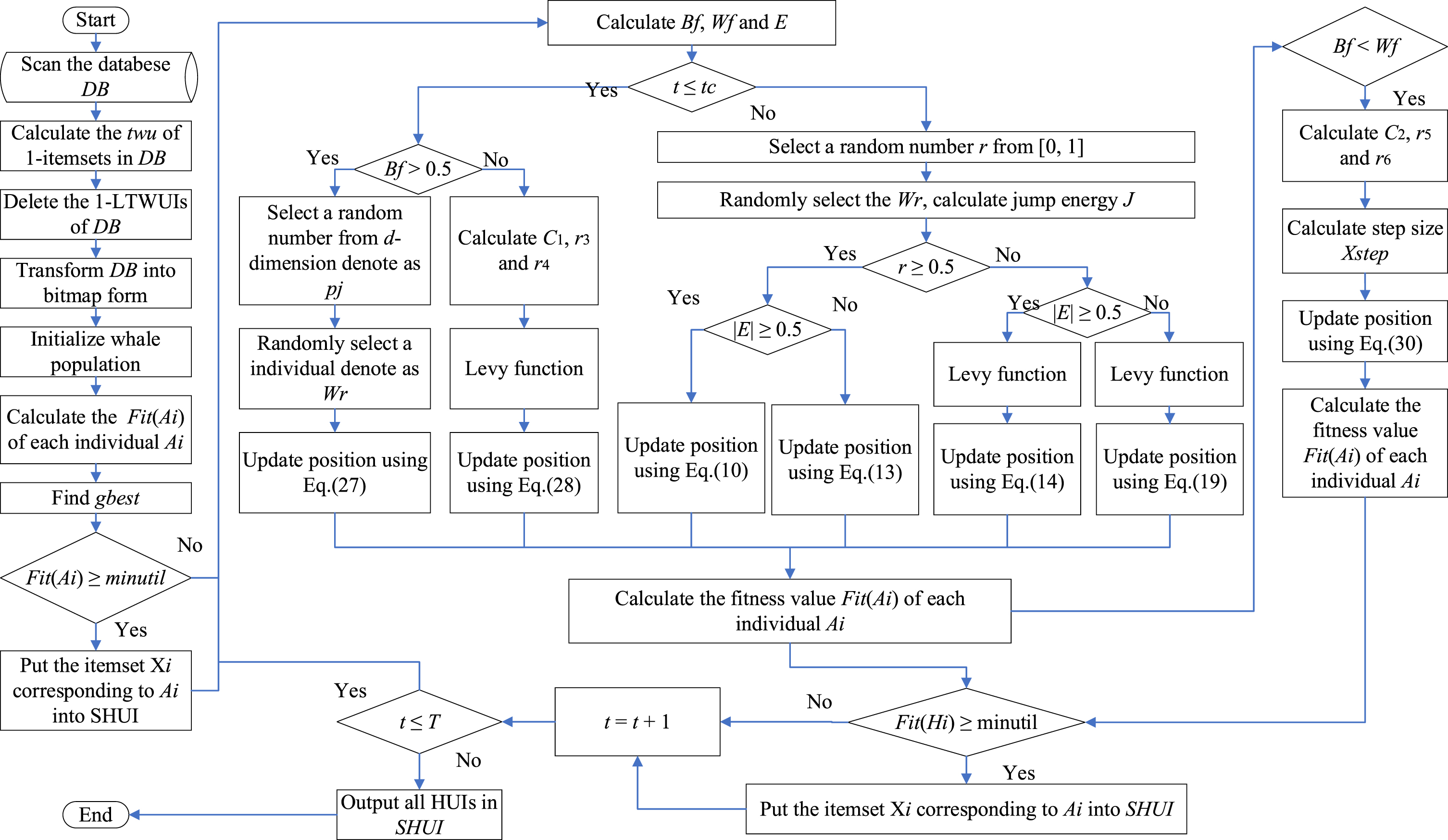
Flowchart of the WHO.

Secondly, the population is initialized, with the number of whales equal to the count of 1-HTWUIs in the dataset. Subsequently, utilizing the WHO algorithm, which hybridizes harris hawk optimization and beluga whale optimization, each individual in the population undergoes multiple iterations to update their positions, generating new individuals.

Finally, the HUIs discovery process is an integral part of each algorithm iteration. For each individual in the population, its fitness function value is computed. The individual with the highest fitness function value from the initial population is selected as the global best (gbest). If the fitness function value of an individual is not less than the minimum utility threshold, its corresponding itemset is considered a high utility itemset and is stored in SHUI (Set of high utility itemsets).

3.3 Algorithm pseudocode

To provide a clearer understanding of the proposed algorithm, here is the pseudocode for the algorithm. Algorithm 1 presents an overview of the algorithm’s general process. Steps 1-2 involve scanning the dataset and removing all 1-itemsets with a twu below the minutil. In step 3, the dataset transforms into a bitmap representation. Step 4 involves the initialization of the population. Step 4 initializes the population by calling the PopulationInitialize () function to initialize pop_size whales. Steps 5 to 12 encompass the core iteration process of the algorithm. In each iteration, the PopulationUpdate() function is invoked to update the positions of the individuals within the population. Subsequently, for each individual after position updates, the FindHUI() function is called to identify valid whales and extract high utility itemsets. In step 10, a comparison is made between the updated population and the original gbest. If an individual with a fitness value surpassing that of gbest is discovered, it is chosen as the new gbest. Step 12 increases the iteration count, initiating a new iteration loop. Upon reaching the maximum iteration count, all high utility itemsets are output.

Algorithm 1 WHO
Input	DB: database, minutil: minimum utility threshold, T: the maximum number of iterations, pop_size: population size
Output	HUIs in DB
1:	scan the data in DB, calculate the TWU of 1-itemsets
2:	remove all 1-LTWUI from DB
3:	transform the database into a bitmap
4:	call PopulationInitialize(); // shown in Algo.2
5:	fort = 1 toTdo
6:	call PopulationUpdate(); // shown in Algo.3
7:	for each whale A_i in population_t do
8:	call FindHUI(); // shown in Algo.4
9:	end for
10:	update the gbest
11:	t = t + 1
12:	end for
13:	output all HUIs

Algorithm 2 presents the pseudocode for population initialization. First, the algorithm takes as input the dataset DB, the number of 1-HTWUIs in the dataset, and the population size. The output is the initial population of whales. First, step 1 creates an empty initial population called “population”. Steps 2 to 8 assign initial positions to each individual in the population. Step 3 creates an empty individual Ai, and steps 4 to 8 represent the initialization process for each whale. The length (dimension) of each whale is equal to the number of 1-HTWUIs in the dataset. For each dimension of each whale, steps 5 to 7 calculate its position. Step 9 adds the whales with their assigned positions to the population. The algorithm iterates until the maximum number of iterations is reached.

Algorithm 2 PopulationInitialize
Input	DB: database, d: the number of 1-HTWUI in DB, pop_size: population size
Output	The first population of whale population
1:	Initialize an empty population list called population
2:	fori = 0 topop_sizedo
3:	Create an empty individual A_i
4:	forj = 0 toddo
5:	p = 2d+3
6:	calculate r(j) using Equation (38)
7:	calculate the position of A_i using
Equation (39)
8:	end for
9:	Add the individual A_i to population
10:	end for

Algorithm 3	PopulationUpdate
Input	population_t_- 1: the old whale population
Output	population_t: the new population
1:	for each whale A_i in population_t_- 1do
2:	Generate a random number r, compute E₀, B_f_,W_f and J using Equation (2) and Equation (7), respectively
3:	if (t≤t_c) then
4:	if (B_f > 0.5) then
5:	Update position using Equation (27) and Equation (22).
6:	else if (B_f≤0.5) then
7:	Update position using Equation (28) and Equation (22).
8:	end if
9:	else if (t > t_c) then
10:	Update the energy E using Equation (6)
11:	if (r≥0.5 and \|E\|≥0.5) then
12:	Update the position of the whale using Equation (10) and Equation (22)
13:	else if (r≥0.5 and \|E\| < 0.5) then
14:	Update the position of the whale using Equation (13) and Equation (22)
15:	else if (r < 0.5 and \|E\|≥0.5) then
16:	Update the position of the whale using Eq. (14) and Eq. (22)
17:	else if (r < 0.5 and \|E\| < 0.5) then
18:	Update the position of the whale using Equation (19) and Equation (22)
19:	end if
20:	end if
21:	if (B_f≤W_f) then
22:	Calculate the step size
23:	Update the position of the whale using Equation (30) and Equation (22)
24:	end if
25:	end for
26:	return population_t

Algorithm 3 outlines the process of population update, taking the old whale population as input and yielding a new whale population as output. For each whale within the old population, steps 2–24 are executed. Initially, step 2 generates a random number to initiate variables. Moving to step 3, a comparison is made between the current iteration count and the predefined iteration count t_c. If t_c has not been reached yet (steps 4–8), step 5 examines whether B_f is greater than 0.5. If affirmative, the exploration phase ensues. The position is updated using equation (27), and continuous variables are transformed into Boolean ones via equation (22). In cases where B_f is less than or equal to 0.5 (steps 6-7), the development phase commences. This involves calculating C₁, generating two random numbers r₃ and r₄, invoking the Levy flight function, and ultimately updating whale positions using equation (28). Subsequently, once the iteration count surpasses t_c, the HHO’s development phase unfolds (steps 10–19). Step 10 sees an update of energy values. The algorithm then leverages a random number r and the absolute value of energy E to determine the subsequent phase. In the algorithm, the whale’s position is updated based on different conditions: when r is greater than or equal to 0.5 and |E| is also greater than or equal to 0.5 (steps 11-12), formulas (10) and (22) are used for the update. When r is greater than or equal to 0.5 but |E| is less than 0.5 (steps 13-14), the update relies on formulas (13) and (22). If r falls below 0.5 while |E| remains at or above 0.5 (steps 15-16), the position is adjusted using formulas (14) and (22). In cases where both r and |E| are less than 0.5 (steps 17-18), the update employs formulas (19) and (22). Furthermore, step 21 involves checking if B_f is less than W_f. If this condition holds true, the algorithm calculates C₂, determines the step size, and proceeds to update the whale’s position using formulas (30) and (22).

Algorithm 4 outlines the functionality of the FindHUI () function, designed to uncover high utility itemsets within the existing whale population. This function takes the current whale population as input and generates a set of high utility itemsets as output. For every whale within the ongoing population, their fitness function value is calculated. In step 3, a comparison is made between the fitness function value of whale A_i and the minimum utility threshold. If this value is greater than or equal to the minimum utility threshold, steps 4-5 proceed by storing the itemset linked to the current whale into SHUI.

Algorithm 4 FindHUI
Input	population_t: the whale population
Output	a set of HUIs SHUI
1:	for each whale A_i in population_tdo
2:	calculate the Fit(A_i)
3:	ifFit(A_i)≥minutil_Wcthen
4:	X_i ← the itemset corresponding to A_i
5:	SHUI ← X_i
6:	end if
7:	end for

3.4 Time complexity of WHO

The proposed WHO consists of three main parts: population initialization, population update, and HUIs discovery. Assume that the population size is n, the maximum number of iterations is T, the dimension of each individual is d, and the time required to compute the fitness function value is timeFit.

Time complexity of population initialization is O(n×k). Time complexity of population update is O(n×d×T). Time complexity of HUIs discovery is O(n×T×timeFit). Then the overall time complexity of WHO is O(n×d + n×d×T + n×T×timeFit) = O(n×T×(d + timeFit)).

4 Experiments

In this chapter, experimental evaluations are carried out from three crucial perspectives: convergence, recall rate, and runtime, aiming to comprehensively assess the efficacy of the proposed algorithm. The experimental datasets encompass chess, connect, mushroom, accidents, foodmart, and retail, each characterized by parameters outlined in Table 5. In which, “No. T” represents the number of transactions, “No. I” represents the number of items, and “Avg. TL” represents the average transaction length.

Table 5
Datasets parameters

datasets No. T No. I Avg. TL Density Type

chess 3196 75 37 49.33 % dense

connect 67557 129 43 33.33 % dense

mushrooms 8416 119 23 19.33 % dense

accidents 340183 468 33.8 7.22 % dense

foodmart 4141 1559 4.42 0.28 % sparse

retail 88162 16470 10.3 0.06 % sparse

datasets	No. T	No. I	Avg. TL	Density	Type
chess	3196	75	37	49.33 %	dense
connect	67557	129	43	33.33 %	dense
mushrooms	8416	119	23	19.33 %	dense
accidents	340183	468	33.8	7.22 %	dense
foodmart	4141	1559	4.42	0.28 %	sparse
retail	88162	16470	10.3	0.06 %	sparse

As shown in Table 6, the experimental environment boasts 15.7GB of available RAM, an Intel Core i9-12900 H @ 2.50 GHz CPU, and operates on the Windows 11 platform. Across all algorithms, the population size is uniformly set to 100, and the upper limit for iterations is established at 1000. The settings of other experiment parameters are shown in Table 7. Given the inherent stochastic nature of intelligent optimization algorithms, leading to notable result variations, all data presented in this section represent averages derived from 10 individual runs.

Table 6

Experimental environment settings

Hardware	CPU	Intel Core i9-12900 H @ 2.50 GHz
environment	RAM	15.7GB
Software	OS	Windows 11
environments	Development	IntelliJ IDEA 2019.2.4 x64
	platform
	Programming Languages	Java

Table 7

Experiment parameters settings

Symbolics	Meanings	Settings
n	population size	100
T	Maximum Iterations	1000
d	Individual size	\|1-HTWUI\|
β	Coefficient of levyFlight	1.5
lb	Lower bounds	0
ub	Upper bounds	1

4.1 Convergence comparison

In this section, we delve into an in-depth comparison of the convergence performance among particle swarm optimization, genetic algorithm, artificial fish swarm algorithm, bat algorithm, and the hybridized WHO algorithm proposed in this paper. To rigorously analyze the convergence trends, a series of experiments were conducted across six datasets. Each algorithm underwent 1000 iterations for every dataset and threshold combination. Figure 3 illustrates the convergence trends of the various algorithms across different datasets and thresholds. The x-axis represents the iteration count, while the y-axis denotes the number of HUIs that each algorithm is capable of uncovering.

Fig. 3

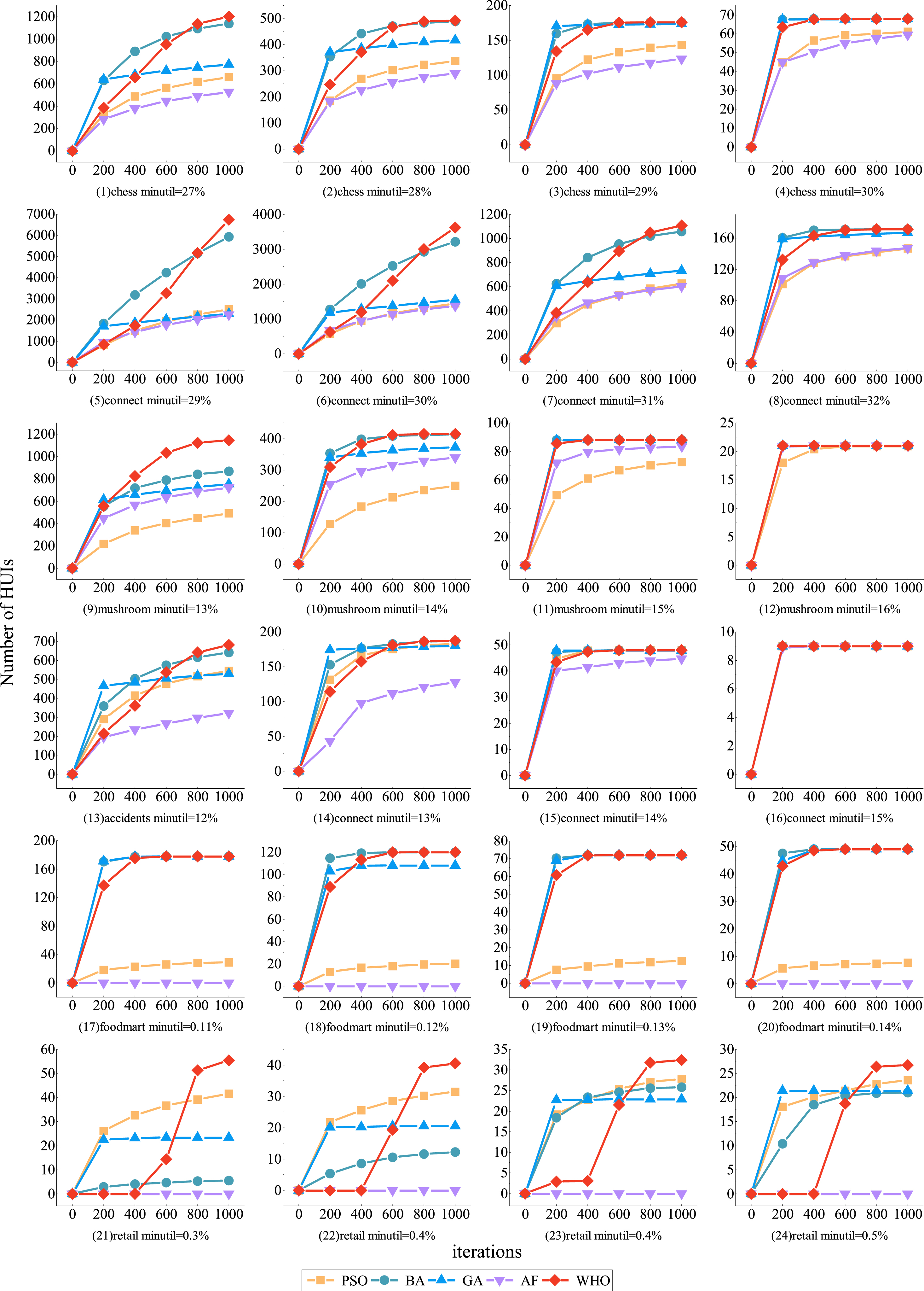
Comparison of Convergence.

Moreover, in the chess dataset, a distinctive trend emerges. When the threshold is set at 27%, the GA demonstrates a notably swifter convergence rate within the initial 0–200 iterations. Nevertheless, beyond 200 iterations and up to 1000, GA’s convergence speed notably decelerates, indicating a potential entrapment in a local optimum around the 200th iteration. Conversely, BA exhibits swift convergence during the 0–600 iteration phase, followed by a somewhat slower pace between 600 and 800 iterations. Notably, both the PSO and AF algorithms maintain a consistently gradual convergence rate, with their final convergence values falling significantly below those achieved by the WHO algorithm. Consequently, they unearth only half the number of HUIs. As the threshold gradually escalates, a general enhancement in the convergence performance of all algorithms becomes evident. This can be attributed to the diminishing count of itemsets meeting the high utility threshold as the threshold value increases, simplifying their swift detection. Remarkably, by the time the threshold reaches 30%, barring AF and PSO, all other algorithms achieve complete convergence before reaching the 200-iteration mark, effectively and efficiently uncovering the entire set of HUIs.

In the connect dataset, when the threshold is set at 29%, the BA demonstrates the highest convergence rate within the 0–600 iterations, followed by the proposed WHO algorithm. However, as the iterations progress into the 600–1000 range, BA’s convergence speed gradually diminishes, and its final convergence value settles around 6000, which is merely 88% of the value achieved by the WHO algorithm. The convergence of the proposed WHO algorithm is optimal between 800 and 1000 iterations, and the number of itemsets continues to grow. If the algorithm’s iteration count could be increased, the WHO algorithm has the potential to uncover even more high utility itemsets beyond this point.

In the mushroom dataset, it is a clear trend emerges that as the threshold increases from 13% to 16%, the WHO algorithm showcases superior convergence performance. Notably, as the threshold rises, the convergence patterns of all algorithms gradually converge as well. When the threshold is set at 13%, the final convergence values achieved by the WHO algorithm are 2.33, 1.32, 1.52, and 1.58 times those of the PSO, BA, GA, and AF algorithms, respectively. Specifically, when the threshold is set at 15%, the WHO, BA, and GA algorithms all achieve complete convergence within the first 400 iterations, whereas the AF and PSO algorithms do not achieve complete convergence. As the threshold elevates to 16%, all algorithms achieve complete convergence within the first 400 iterations.

In the accidents dataset, when the threshold is set at 12%, the GA displays the swiftest convergence rate during the initial 0–200 iterations, closely followed by the BA. However, as the number of iterations surpasses 600, both GA and BA gradually become ensnared in local optima. At 13% and 14% thresholds, except for the underperforming AF algorithm, the remaining algorithms showcase commendable convergence performance. Upon reaching a 15% threshold, all algorithms manage to achieve their maximum convergence values within the first 200 iterations.

In the foodmart dataset, as the threshold increases from 0.11% to 0.14%, the algorithm with the best convergence performance is BA, with the WHO algorithm closely following behind BA. Conversely, the PSO algorithm demonstrates relatively subpar convergence, while the AF algorithm exhibits the weakest convergence performance. This discrepancy can be attributed to the sparse characteristics of the foodmart dataset, where the AF algorithm’s runtime extends beyond 24 hours without completing the initial 200 iterations, thereby hindering the acquisition of conclusive experimental outcomes.

In the retail dataset, although the WHO algorithm initially exhibits slightly slower convergence performance compared to the PSO, GA, and BA algorithms, its convergence speed significantly accelerates during the iterations ranging from 600 to 1000. Furthermore, the WHO algorithm ultimately achieves a far higher convergence value than the other comparative algorithms.

4.2 Recall rate comparison

By comparing the quantities of high utility itemsets discovered through different algorithms, we can conduct a comprehensive analysis of their recall rates. Table 8 outlines the recall rates for each algorithm. Notably, across all datasets, as the threshold is increased, the recall rates of the algorithms steadily rise. This phenomenon is a result of the diminishing count of itemsets meeting the minimum utility threshold as the threshold value increases. As a consequence, algorithms can more readily identify a greater number, or even the entirety, of high utility itemsets.

Table 8
Recall comparison (Bold indicates the best, and the number inside parentheses represents the algorithm’s ranking.)

datasets minutil(%) WHO PSO BA GA AF

chess 27 96.48% (1) 52.89% (4) 91.36% (2) 62.04% (3) 42.22% (5)

28 99.86% (1) 68.36% (4) 99.23% (2) 84.58% (3) 58.82% (5)

29 100.00% (1) 81.25% (4) 100.00% (1) 98.30% (3) 69.89% (5)

30 100.00% (1) 89.71% (4) 100.00% (1) 98.53% (3) 86.76% (5)

connect 29 36.84% (1) 13.71% (3) 32.46% (2) 12.57% (4) 12.29% (5)

30 68.83% (1) 27.40% (4) 61.04% (2) 29.26% (3) 26.02% (5)

31 96.83% (1) 54.72% (4) 92.51% (2) 64.23% (3) 52.71% (5)

32 100.00% (1) 85.38% (5) 100.00% (1) 97.37% (3) 85.96% (4)

mushroom 13 99.38% (1) 42.62% (5) 75.34% (2) 65.37% (3) 62.78% (4)

14 100.00% (1) 60.00% (5) 99.64% (2) 89.83% (3) 81.93% (4)

15 100.00% (1) 81.82% (5) 100.00% (1) 100.00% (1) 94.32% (4)

16 100.00% (1) 95.24% (5) 100.00% (1) 100.00% (1) 100.00% (1)

accidents 12 93.64% (1) 74.73% (3) 88.17% (2) 72.66% (4) 44.23% (5)

13 99.21% (1) 96.83% (3) 98.94% (2) 94.71% (4) 70.90% (5)

14 100.00% (1) 100.00% (1) 100.00% (1) 97.92% (4) 91.67% (5)

15 100.00% (1) 100.00% (1) 100.00% (1) 100.00% (1) 100.00% (1)

foodmart 0.11 100.00% (1) 16.29% (4) 100.00% (1) 100.00% (1) 0.00% (5)

0.12 100.00% (1) 24.17% (4) 100.00% (1) 90.00% (3) 0.00% (5)

0.13 100.00% (1) 16.67% (4) 100.00% (1) 100.00% (1) 0.00% (5)

0.14 100.00% (1) 14.29% (4) 100.00% (1) 100.00% (1) 0.00% (5)

retail 0.3 93.90% (1) 69.49% (2) 8.47% (4) 38.98% (3) 0.00% (5)

0.4 98.78% (1) 75.61% (2) 29.27% (4) 48.78% (3) 0.00% (5)

0.5 98.18% (1) 81.82% (2) 75.76% (3) 66.67% (4) 0.00% (5)

0.6 98.89% (1) 85.19% (2) 77.78% (3) 77.78% (3) 0.00% (5)

Average rank 1.00 3.54 1.88 2.71 4.50

datasets	minutil(%)	WHO	PSO	BA	GA	AF
chess	27	96.48% (1)	52.89% (4)	91.36% (2)	62.04% (3)	42.22% (5)
	28	99.86% (1)	68.36% (4)	99.23% (2)	84.58% (3)	58.82% (5)
	29	100.00% (1)	81.25% (4)	100.00% (1)	98.30% (3)	69.89% (5)
	30	100.00% (1)	89.71% (4)	100.00% (1)	98.53% (3)	86.76% (5)
connect	29	36.84% (1)	13.71% (3)	32.46% (2)	12.57% (4)	12.29% (5)
	30	68.83% (1)	27.40% (4)	61.04% (2)	29.26% (3)	26.02% (5)
	31	96.83% (1)	54.72% (4)	92.51% (2)	64.23% (3)	52.71% (5)
	32	100.00% (1)	85.38% (5)	100.00% (1)	97.37% (3)	85.96% (4)
mushroom	13	99.38% (1)	42.62% (5)	75.34% (2)	65.37% (3)	62.78% (4)
	14	100.00% (1)	60.00% (5)	99.64% (2)	89.83% (3)	81.93% (4)
	15	100.00% (1)	81.82% (5)	100.00% (1)	100.00% (1)	94.32% (4)
	16	100.00% (1)	95.24% (5)	100.00% (1)	100.00% (1)	100.00% (1)
accidents	12	93.64% (1)	74.73% (3)	88.17% (2)	72.66% (4)	44.23% (5)
	13	99.21% (1)	96.83% (3)	98.94% (2)	94.71% (4)	70.90% (5)
	14	100.00% (1)	100.00% (1)	100.00% (1)	97.92% (4)	91.67% (5)
	15	100.00% (1)	100.00% (1)	100.00% (1)	100.00% (1)	100.00% (1)
foodmart	0.11	100.00% (1)	16.29% (4)	100.00% (1)	100.00% (1)	0.00% (5)
	0.12	100.00% (1)	24.17% (4)	100.00% (1)	90.00% (3)	0.00% (5)
	0.13	100.00% (1)	16.67% (4)	100.00% (1)	100.00% (1)	0.00% (5)
	0.14	100.00% (1)	14.29% (4)	100.00% (1)	100.00% (1)	0.00% (5)
retail	0.3	93.90% (1)	69.49% (2)	8.47% (4)	38.98% (3)	0.00% (5)
	0.4	98.78% (1)	75.61% (2)	29.27% (4)	48.78% (3)	0.00% (5)
	0.5	98.18% (1)	81.82% (2)	75.76% (3)	66.67% (4)	0.00% (5)
	0.6	98.89% (1)	85.19% (2)	77.78% (3)	77.78% (3)	0.00% (5)
Average rank		1.00	3.54	1.88	2.71	4.50

In the chess dataset, the proposed WHO algorithm exhibits the highest recall rate. Specifically, within the threshold range of 29–30%, it achieves a remarkable 100% recall rate, effectively capturing all the high utility itemsets present in the dataset. Even at a threshold of 27%, the WHO algorithm maintains a robust recall rate of 96.48%, with only a marginal number of itemsets being missed. Furthermore, WHO outperforms other algorithms by discovering high utility itemsets 2.29 times more than AF, 1.82 times more than PSO, and 1.56 times more than GA. The second-highest recall rate is observed with the BA algorithm.

In the case of the connect dataset, at a threshold of 29%, the algorithms attain a peak recall rate of 36.84%. This can be attributed to the dataset’s unique attributes— comprising a substantial 67,557 transactions and 129 items— resulting in a sizable and dense dataset. Given the constraint of 1000 iterations, the algorithms face a challenge in unearthing a large quantity of HUIs within such a dense data space. Extending the iteration count might enhance the recall rate further. As depicted in Table 5, the WHO algorithm boasts the highest recall rate, closely followed by BA. Particularly noteworthy is that at a 30% threshold, the WHO algorithm outperforms PSO, AF, BA, and GA in recall rate by factors of 2.51, 2.65, 1.13 and 2.35, respectively. Upon raising the threshold to 32%, only WHO and BA succeed in achieving a flawless 100% recall rate, indicating their capability to uncover the entirety of high utility itemsets at that juncture.

In the mushroom dataset, it is quite apparent that the WHO algorithm boasts the highest recall rate. At a threshold of 13%, it achieves an impressive recall rate of 99.38%, and this rate increases to 100% as the threshold continues to rise. Furthermore, with a threshold of 15%, not only WHO but also the BA and GA algorithms achieve a perfect 100% recall rate. Similarly, when the threshold climbs to 16%, the AF algorithm’s recall rate also reaches a flawless 100%.

In the accidents dataset, the WHO algorithm demonstrates the highest recall rate, followed by PSO, BA, GA, and AF. At a threshold of 12%, the recall rate of WHO is 1.25 times that of PSO, 2.12times that of AF, 1.06 times that of BA, and 1.29 times that of GA.

In the foodmart dataset, both the WHO and BA algorithms achieve a 100% recall rate, meaning they can mine all the high utility itemsets present in the dataset. In contrast, the AF algorithm has a recall rate of 0% because it runs for more than 24 hours without obtaining any high utility itemsets.

For the retail dataset, the WHO algorithm achieves the highest recall rate. At a threshold of 0.3%, the recall rate of WHO is 1.35 times that of PSO, 11.08 times that of BA, and 2.41 times that of GA. Similarly, at a threshold of 0.4%, the recall rate of WHO is 1.31 times that of PSO, 3.38 times that of BA, and 2.03 times that of GA. At a threshold of 0.5%, the recall rate of WHO is 1.20 times that of PSO, 1.30 times that of BA, and 1.47 times that of GA. Finally, at a threshold of 0.6%, the recall rate of WHO is 1.16 times that of PSO, 1.27 times that of BA, and 1.27 times that of GA.

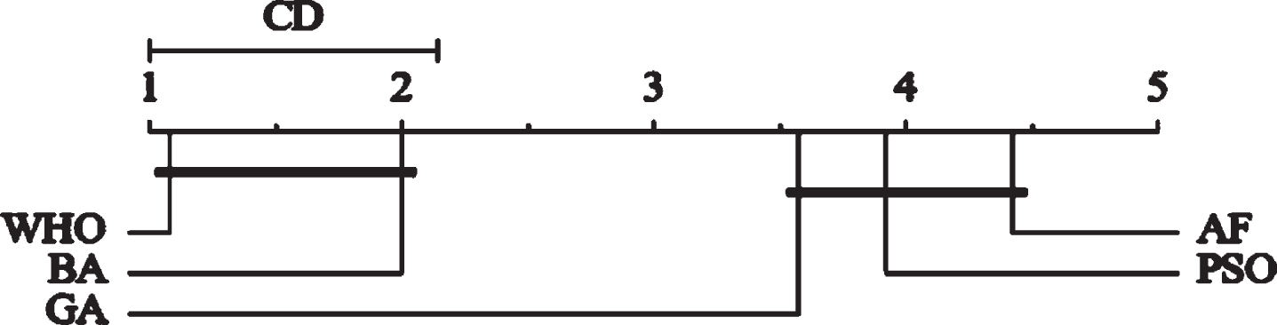
We performed a nonparametric statistical significance test on the experimental data. Figure 4 shows the Bonferroni-Dunn statistical analysis of Recall. where the CD value is calculated as in Eq. (40), where q_α is fixed to 2.498, k is the number of algorithms, and N is the size of the dataset. In this paper, k is taken as 5 and N is 24, so the CD is calculated as 1.14.

Fig. 4

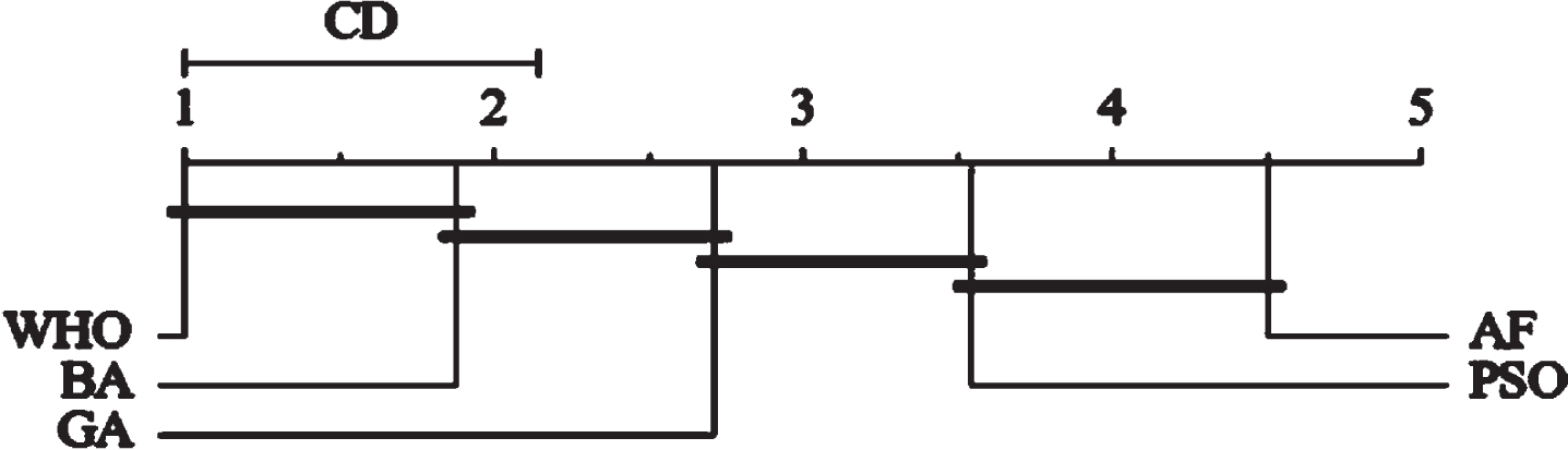
Bonferroni-Dunn statistical analysis on Recall.

$CD = q_{α} \sqrt{\frac{k (k + 1)}{6 N}}$ (40)

From the figure, it can be seen that the proposed algorithm WHO is significantly different from the three algorithms except BA. According to Equation (40), when the number of algorithms is 5, the number of datasets N is taken as 32 in order to make the CD value less than 1. While the algorithm WHO has been ranked first and the average ranking of BA is 1.88, so it does not have a significant difference, but WHO is significantly better than BA.

4.3 Runtime comparison

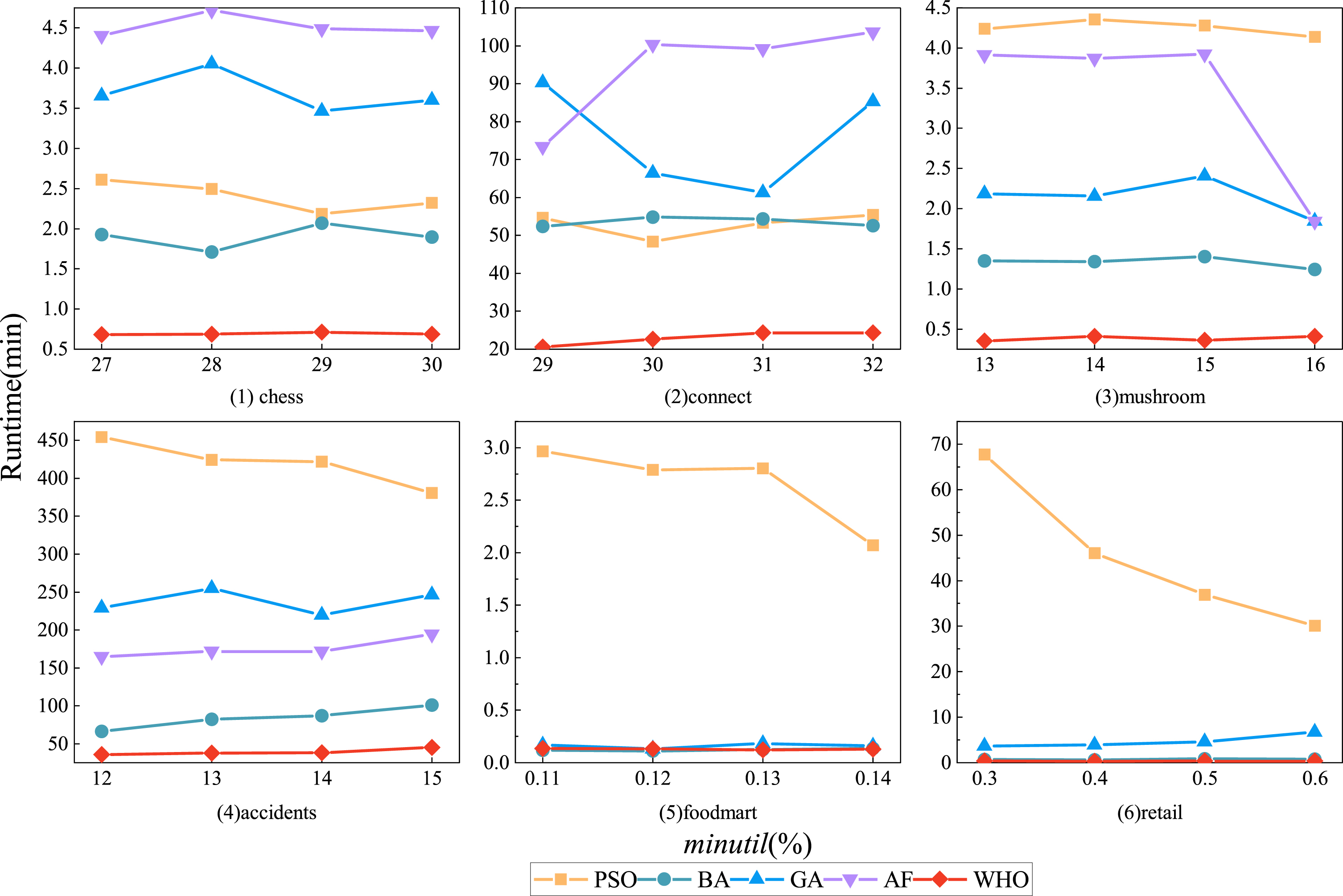
In this subsection, we delve into the comparison of algorithm runtimes. Figure 3 provides insight into the trend of algorithm runtimes as they vary with different thresholds.

Notably, the AF algorithm’s runtime exceeded 24 hours for the sparse datasets foodmart and retail, without yielding any results, hence, it’s not depicted in the figure. Unlike traditional methods for mining high utility itemsets, the runtime of intelligent optimization-based algorithms doesn’t decrease with increasing thresholds. Instead, it exhibits a higher degree of stability. This phenomenon is mainly attributed to the fact that the runtime of intelligent optimization-based algorithms is primarily influenced by factors such as the maximum iteration count and the approach used to update the population, with a lesser dependency on the threshold.

In the chess dataset, Algorithm WHO stands out with a lower runtime compared to the other comparative algorithms. Specifically, the runtime ratios of PSO, BA, GA, and AF to WHO are 3.47, 2.74, 5.33 and 6.52, respectively. Moving to the connect dataset, Algorithms WHO, BA and PSO maintain relatively stable runtimes, while AF and GA experience more noticeable fluctuations as the threshold varies. The runtime ratios of PSO, BA, GA, and AF to WHO are 2.31, 2.33, 3.31 and 4.10, respectively. In the mushroom dataset, Algorithms WHO, BA and PSO exhibit higher runtime stability, followed by GA. Notably, AF’s runtime fluctuates largely as the threshold shifts from 15% to 16%. The runtime ratios of PSO, BA, GA, and AF to WHO are 11.08, 3.47, 5.59 and 8.82, respectively. Shifting focus to the accidents dataset, WHO maintains the lowest runtime, followed by BA, AF, GA, and PSO, with runtime ratios of 10.73, 2.15, 6.06 and 4.49 to WHO, respectively. In the sparse foodmart dataset, all algorithms, except for PSO, boast relatively low runtimes and are capable of completing iterations within one minute. Finally, in the retail dataset, Algorithm WHO again showcases the lowest runtime, with PSO’s runtime being 120.76 times that of WHO.

Next the nonparametric statistical significance test of Runtime of the algorithm is performed using Bonferroni-Dunn method. Table 9 shows the runtimes of the algorithms along with their rankings. Figure 5 shows the Bonferroni-Dunn statistical analysis of Runtime. As can be seen from the figure, the proposed algorithm WHO significantly outperforms the algorithms GA, PSO as well as AF. When compared to the algorithm BA, although there is no significance difference, the WHO’s runtime is significantly better than BA in general.

Fig. 5

Bonferroni-Dunn statistical analysis on Runtime.

Table 9

Runtime(min)

datasets	minutil(%)	WHO	PSO	BA	GA	AF
chess	27	0.68 (1)	2.61 (3)	1.93 (2)	3.65 (4)	4.40 (5)
	28	0.69 (1)	2.49 (3)	1.71 (2)	4.05 (4)	4.72 (5)
	29	0.71 (1)	2.19 (3)	2.07 (2)	3.46 (4)	4.49 (5)
	30	0.69 (1)	2.32 (3)	1.90 (2)	3.60 (4)	4.47 (5)
connect	29	20.54 (1)	54.59 (3)	52.41 (2)	90.31 (5)	73.44 (4)
	30	22.61 (1)	48.39 (2)	54.85 (3)	66.48 (4)	100.33 (5)
	31	24.29 (1)	53.30 (2)	54.32 (3)	61.25 (4)	99.19 (5)
	32	24.32 (1)	55.36 (3)	52.54 (2)	85.33 (4)	103.59 (5)
mushroom	13	0.35 (1)	4.24 (5)	1.35 (2)	2.18 (3)	3.91 (4)
	14	0.41 (1)	4.35 (5)	1.34 (2)	2.15 (3)	3.87 (4)
	15	0.36 (1)	4.28 (5)	1.40 (2)	2.41 (3)	3.92 (4)
	16	0.41 (1)	4.14 (5)	1.24 (2)	1.84 (4)	1.84 (3)
accidents	12	35.77 (1)	454.39 (5)	66.38 (2)	229.02 (4)	165.06 (3)
	13	37.62 (1)	424.49 (5)	82.04 (2)	255.04 (4)	171.80 (3)
	14	38.21 (1)	422.13 (5)	86.76 (2)	219.56 (4)	171.69 (3)
	15	45.09 (1)	380.54 (5)	101.25 (2)	246.54 (4)	194.21 (3)
foodmart	0.11	0.14 (2)	2.96 (4)	0.12 (1)	0.17 (3)	– (5)
	0.12	0.13 (2)	2.79 (4)	0.11 (1)	0.13 (3)	–(5)
	0.13	0.12 (1)	2.80 (4)	0.13 (2)	0.18 (3)	– (5)
	0.14	0.13 (1)	2.07 (4)	0.14 (2)	0.16 (3)	– (5)
retail	0.3	0.38 (1)	67.69 (4)	0.73 (2)	3.70 (3)	–(5)
	0.4	0.34 (1)	46.03 (4)	0.66 (2)	3.91 (3)	–(5)
	0.5	0.43 (1)	36.95 (4)	0.88 (2)	4.64 (3)	–(5)
	0.6	0.36 (1)	30.11 (4)	0.78 (2)	6.70 (3)	–(5)
Average rank		1.08	3.92	2.00	3.58	4.42

For memory usage, it is primarily influenced by the population size and the dimensionality of individuals in terms of space. When the population size is the same, the memory consumption of various algorithms is not significantly different, so no comparison is made.

In the subsequent analysis, we conduct a performance comparison of the proposed WHO algorithm and the hybrid DE-BGWO algorithm in terms of two key aspects: execution time and recall rate. Figure 4 provides a visual representation of the execution time comparison. As depicted in Fig. 7, it is evident that the WHO algorithm demonstrates considerably shorter execution times in comparison to the DE-BGWO algorithm. This observation underscores the superior efficiency of the WHO algorithm in terms of computational speed.

Fig. 6

Comparison of Runtime.

Fig. 7

Comparison of runtime with DE-BGWO.

In connect dataset, when the threshold is set at 31.2%, the DE-BGWO algorithm takes 22492 seconds to complete the mining process, whereas the proposed WHO algorithm accomplishes the task in just 1362 seconds, representing approximately 7% of the DE-BGWO algorithm’s runtime. When the threshold is raised to 31.4%, the DE-BGWO algorithm requires 23552 seconds to run, while the WHO algorithm runs for 1303 seconds, roughly 6% of the DE-BGWO algorithm’s runtime. As the threshold increases to 31.6%, the WHO algorithm operates for 1520 seconds, whereas DE-BGWO takes 25276 seconds, making DE-BGWO approximately 16.63 times slower than WHO. At a threshold of 31.8%, the WHO algorithm runs for 1533 seconds, while DE-BGWO runs for 23944 seconds, making DE-BGWO roughly 15.62 times slower than WHO. Finally, with a threshold of 32%, the WHO algorithm completes its process in 1459 seconds, whereas DE-BGWO takes 23909 seconds, making DE-BGWO approximately 16.38 times slower than WHO.

In the accident 8% dataset, when the thresholds are set at 13.3%, 13.5%, 13.7%, 13.9%, and 14.1%, the DE-BGWO algorithm’s runtimes are 53.35, 54.89, 53.22, 54.18, and 55.40 times longer than that of the WHO algorithm, respectively. This indicates that the proposed WHO algorithm not only improves efficiency but also offers significant time savings for handling large-scale tasks. It is particularly well-suited for complex tasks that require efficient processing.

In the chess dataset, the DE-BGWO algorithm’s average runtime is 61.27 times longer than that of the WHO algorithm. When the thresholds are set at 28.3%, 28.5%, 28.7%, 28.9%, and 30.1%, the WHO algorithm’s runtimes are 1.68%, 1.86%, 1.56%, 1.54%, and 1.56% of the DE-BGWO algorithm’s runtime, respectively.

In the mushroom dataset, the DE-BGWO algorithm’s average runtime is 53.74 times longer than that of the WHO algorithm. When the thresholds are set at 14.2%, 14.4%, 14.6%, 14.8%, and 15%, the WHO algorithm’s runtimes are 2.15%, 1.92%, 1.67%, 1.83%, and 1.79% of the DE-BGWO algorithm’s runtime, respectively.

Table 10 presents an analysis of the recall rates for the proposed WHO algorithm and the DE-BGWO algorithm. The recall rate of an algorithm is calculated as the ratio of the number of HUIs mined by the algorithm to the total number of HUIs in the dataset.

Table 10

Comparison of recall rate with DE-BGWO

	minutil(%)	DE-BGWO	WHO
connect	31.2	99.98	98.43
	31.4	99.91	99.65
	31.6	99.95	99.95
	31.8	99.78	100.00
	32	99.38	100.00
accident_8%	13.3	99.91	100.00
	13.5	99.43	100.00
	13.7	99.83	100.00
	13.9	99.95	100.00
	14.1	99.92	100.00
chess	28.3	98.92	100.00
	28.5	99.87	100.00
	28.7	98.85	100.00
	28.9	99.95	100.00
	30.1	99.89	100.00
mushroom	14.2	99.56	100.00
	14.4	99.34	100.00
	14.6	99.9	100.00
	14.8	99.89	100.00
	15	99.78	100.00

From the table, we observe that in the connect dataset, when the thresholds are set at 31.2% and 31.4%, the recall rate of the WHO algorithm is 1.55% and 0.26% lower than that of the DE-BGWO algorithm, respectively. At a threshold of 31.6%, both algorithms achieve the same recall rate of 99.95%. When the threshold is increased to 31.8% and 32%, the WHO algorithm reaches a 100% recall rate, while the DE-BGWO algorithm achieves recall rates of 99.78% and 99.38%, respectively. In the accident 8%, chess, and mushroom datasets, the WHO algorithm is able to mine all high utility itemsets with a recall rate of 100%, while the DE-BGWO algorithm falls short of achieving a 100% recall rate.

4.4 Result and discussion

In this Chapter, the performance of the proposed WHO is evaluated in terms of convergence, recall rate, and Runtime.

For convergence, the algorithm WHO has the best convergence performance in chess, connect, mushroom, accidents, retail. And the convergence performance in foodmart dataset is ranked 3rd. This is because the average transaction length of the foodmart dataset is 4.42, the distribution of the HUIs is very decentralized, and the proposed method WHO requires extensive exploration to find the HUIs in the initial run of the algorithm. Therefore, one of the advantages of WHO is good convergence performance. The disadvantage is slightly poor convergence in datasets that are too sparse and have a small average transaction length.

In terms of recall rate, the proposed WHO achieves the highest recall rate across all datasets. This indicates that the proposed algorithm has high mining capability and good convergence, and is able to mine a larger number of HUIs in a limited time.

In terms of runtime, in the remaining five datasets except foodmart dataset, the running time of the proposed WHO is much shorter than the other compared algorithms and has the best stability. This indicates that this study can effectively improve the mining efficiency of the algorithm. Therefore, the additional advantages of the proposed WHO are higher efficiency and the runtime is less affected by the threshold value.

In summary, this study can effectively solve the problem that the heuristic-based HUIM algorithms are easy to trap in local optimum, which leads to a large number of missing itemsets. Additionally, this study improves the efficiency of heuristic-based HUIM methods.

High utility itemsets mining has widespread real-world applications in various domains, including retail, e-commerce, market basket analysis, healthcare, logistics and supply chain management, social networks, finance, production, and manufacturing, among others. In the retail industry, it assists businesses in optimizing inventory management and promotional strategies. E-commerce platforms can increase sales volume and customer satisfaction through it. In the healthcare sector, it can be utilized for disease factor analysis. In the financial sector, it can be employed for risk management and transaction analysis. In the realm of social networks, it can be utilized for content recommendation and targeted advertising. These are just a few of the many real-world application areas where HUIM provides valuable insights and assistance across industries.

5 Conclusion

High utility itemsets mining aims to mine out significant itemsets in the transaction database. In recent years, heuristic algorithms have been widely used in HUIM. In order to solve the problem that the current heuristic-based HUIM method is easy to fall into local optimization and lose a large number of itemsets. This paper proposes a new intelligent optimization algorithm that integrates harris hawk optimization and beluga whale optimization. The initialization strategy of whales based on good point set is proposed and designed, which helps to improve the diversity of the population and can improve the shortcomings of poor quality and stability of the population, which is easy to fall into the local optimization. In order to test the performance of the proposed algorithm, a large number of experiments are conducted on six real datasets of chess, connect, mushroom, accidents, foodmart, and retail in terms of convergence, recall rate, and runtime of the algorithm. Experimental results show that the proposed algorithm outperforms the current state-of-the-art heuristic-based HUIM algorithms. It can be concluded that the advantages of the proposed algorithm WHO are good convergence performance; high mining capability, good convergence, higher efficiency and the runtime is less affected by the threshold value. The disadvantages are slightly poor convergence in datasets that are too sparse and have a small average transaction length. In the future, our research group will continue to develop more efficient heuristic-based HUIM algorithms, like ant lion optimization (ALO) [51]-based and GWO [10]-based HUIM algorithms.

Funding

This work was supported by the National Nature Science Foundation of China (62062004) and the Ningxia Natural Science Foundation Project (2023AAC03315).

Author contributions

Zhihui Gao and Meng Han wrote the main manuscript text. Shujuan Liu, Ang Li and Dongliang Mu helped revise the manuscript format and collect data. All authors reviewed the manuscript.

References

Lin

J.C.W.

, Djenouri

, Srivastava

and Fourier-Viger

, Efficient evolutionary computation model of closed high-utility itemset mining, Applied Intelligence 52(9) (2022), 10604–10616.

Liu

, Qu

Mining high utility itemsets without candidate generation, in: the 21st ACM international conference on Information and knowledge management, (2012), 55–64.

Zida

, Fournier-viger

, Lin

J.C.W.

, Wu

W.C.

and Tseng

V.S.

, EFIM: a fast and memory efficient algorithm for high-utility itemset mining, Knowledge and Information Systems 51(2) (2017), 595–625.

Fournier-viger

, Wu

C.W.

, Zida

, Tseng

V.S.

FHM: Faster high-utility itemset mining using estimated utility co-occurrence pruning, in: the Foundations of Intelligent Systems: 21st International Symposium, (2014), 83–92.

Cheng

, Fang

, Shen

, Lin

J.C.W.

and Yuan

, An efficient utility-list based high-utility itemset mining algorithm, Applied Intelligence 53(6) (2023), 6992–7006.

Nawaz

M.S.

, Fournier-viger

, Yun

, Wu

and Song

, Mining high utility itemsets with hill climbing and simulated annealing, ACM Transactions on Management Information System 13(1) (2021), 1–22.

Vanchinathan

, Valluvan

K.R.

, Gnanavel

and Gokul

, Numerical simulation and experimental verification offractional-order PIλ controller for solar PV fed sensorless brushless DC motor using whale optimizationalgorithm, Electric Power Components and Systems 50(1-2) (2022), 64–80.

Ala

, Mahmoudi

, Mirjalili

, Simic

and Pamucar

, Evaluating the Performance of various Algorithms for Wind Energy Optimization: A Hybrid Decision-Making model, Expert Systems with Applications 221 (2023), 119731–119751.

Ala

, Yazdani

, Ahmadi

, Poorianasab

and Attari

M.Y.N.

, An efficient healthcare chain design for resolving the patient scheduling problem: queuing theory and MILP-ASA optimization approach, Annals of Operations Research 328 (2023), 3–33.

10.

Ala

, Simic

, Pamucar

and Jana

, A Novel Neutrosophic-Based Multi-Objective Grey Wolf Optimizer for Ensuring the Security and Resilience of Sustainable Energy: A Case Study of Belgium, Sustainable Cities and Society 96 (2023), 104709–104727.

11.

Kannimuthu

and Premalatha

, Discovery of high utility itemsets using genetic algorithm with ranked mutation, Applied Artificial Intelligence 28(4) (2014), 337–359.

12.

Lin

W.J.C.

, Yang

, Fournier-Viger

, Hong

T.P.

and Voznak

, A binary PSO approach to mine high-utility itemsets, Soft Computing 21 (2017), 5103–5121.

13.

Song

, Huang

Discovering high utility itemsets based on the artificial bee colony algorithm, in: Advances in Knowledge Discovery and Data Mining, (2018), 3–14.

14.

Song

, Li

, Huang

Artificial fish swarm algorithm for mining high utility itemsets, in: Advances in Swarm Intelligence: 12th International Conference, (2021), 407–419.

15.

Pazhaniraja

, Sountharrajan

, Suganya

and Karthiga

, Optimizing high-utility item mining using hybrid dolphin echolocation and Boolean grey wolf optimization, Journal of Ambient Intelligence and Humanized Computing 14(3) (2023), 2327–2339.

16.

Song

and Huang

, Mining high average-utility itemsets based on particle swarm optimization, Data Science and Pattern Recognition 4(2) (2020), 19–32.

17.

Lin

W.J.C.

, Djenouri

, Srivastava

, Yun

and Fournier-Viger

, A predictive GA-based model for closed high-utility itemset mining, Applied Soft Computing 108 (2021), 107422–107430.

18.

Song

, Zheng

, Huang

and Liu

, Heuristically mining the top-k high-utility itemsets with cross-entropy optimization, Applied Intelligence 52 (2021), 17026–17041.

19.

Luna

J.M.

, Kiran

R.U.

, Fournier-Viger

and Ventura

, Efficient mining of top-k high utility itemsets through genetic algorithms, Information Sciences 624 (2023), 529–553.

20.

Song

and Huang

, Mining high utility itemsets using bio-inspired algorithms: A diverse optimal value framework, IEEE Access 6 (2018), 19568–19582.

21.

Zhang

, Fang

, Sun

and Wang

, Improved genetic algorithm for high-utility itemset mining, IEEE Access 7 (2019), 176799–176813.

22.

Lin

J.C.W.

, Djenouri

, Srivastava

and Fourier-Viger

, Efficient evolutionary computation model of closed high-utility itemset mining, Applied Intelligence 52(9) (2022), 10604–10616.

23.

Dam

T.L.

, Li

, Fournier-Viger

and Duong

Q.H.

, CLS-Miner: efficient and effective closed high-utility itemset mining, Frontiers of Computer Science 13 (2019), 357–381.

24.

Lin

J.C.W.

, Yang

, Fournier-Viger

, Wu

J.M.T.

, Hong

T.P.

, Wang

L.S.L.

and Zhan

, Mining high-utility itemsets based on particle swarm optimization, Engineering Applications of Artificial Intelligence 55 (2016), 320–330.

25.

Wang

C.W.

, Yin

S.L.

, Liu

W.Y.

, Wei

X.M.

, Zheng

H.J.

and Yang

J.P.

, High Utility Itemset Mining Algorithm Based on Improved Particle Swarm Optimization, Journal of Chinese Computer Systems 41(5) (2020), 1084–1090.

26.

Song

, Li

Discovering high utility itemsets using set-based particle swarm optimization, in: Advanced Data Mining and Applications: 16th International Conference, (2020), 38–53.

27.

Fang

, Zhang

, Lu

and Lin

J.C.W.

, High-utility itemsets mining based on binary particle swarm optimization with multiple adjustment strategies, Applied Soft Computing 124 (2022), 109073–109084.

28.

Subramanian

, Kandhasamy

Mining high utility itemsets using Genetic Algorithm Based-Particle Swarm Optimization (GA-PSO), Journal of Intelligent & Fuzzy Systems, (Preprint) (2023), 1–21.

29.

Logeswaran

, Suresh

and Anandamurugan

, Particle Swarm Optimization Method Combined with off Policy Reinforcement Learning Algorithm for the Discovery of High Utility Itemset, Information Technology and Control 52(1) (2023), 25–36.

30.

Gunawan

, Winarko

and Pulungan

, Performance comparison of inertia weight and acceleration coefficients of BPSO in the context of high-utility itemset mining, Evolutionary Intelligence 16(3) (2023), 943–961.

31.

Yang

, Ding

, Wang

, Xing

and Li

, A High Utility ItemsetMining Algorithm Based on Particle Filter, MathematicalProblems in Engineering 2023 (2023), 1–15.

32.

Sukanya

N.S.

and Thangaiah

P.R.J.

, Enhanced differential evolution and particle swarm optimization approaches for discovering high utility itemsets, International Journal of Computational Intelligence and Applications 22(01) (2023), 2341005–2341022.

33.

Gunawan

, Winarko

and Pulungan

, A BPSO-based method for high-utility itemset mining without minimum utility threshold, Knowledge-Based Systems 190 (2020), 105164–105211.

34.

J.M.T.

, Zhan

and Lin

J.C.W.

, An ACO-based approach to mine high-utility itemsets, Knowledge-Based Systems 116 (2017), 102–113.

35.

Arunkumar

M.S.

, Suresh

and Gunavathi

, High utility infrequent itemset mining using a customized ant colony algorithm, International Journal of Parallel Programming 48 (2020), 833–849.

36.

Pramanik

and Goswami

, Discovery of closed high utility itemsets using a fast nature-inspired ant colony algorithm, Applied Intelligence 52(8) (2022), 8839–8855.

37.

Pazhaniraja

, Sountharrajan

and Sathis

, Kumar, High utility itemset mining: a Boolean operators-based modified grey wolf optimization algorithm, Soft Computing 24 (2020), 16691–16704.

38.

Pazhaniraja

and Sountharrajan

, High utility itemset mining using dolphin echolocation optimization, Journal of Ambient Intelligence and Humanized Computing 12 (2021), 8413–8426.

39.

Krishna

G.J.

and Ravi

, Mining top high utility association rulesusing binary differential evolution, Engineering Applicationsof Artificial Intelligence 96 (2020), 103935–103951.

40.

Krishna

G.J.

and Ravi

, High utility itemset mining using binary differential evolution: An application to customer segmentation, Expert Systems with Applications 181 (2021), 115122–115134.

41.

Zhang

, Fu

, Cheng

, Qiu

and Su

, A multi-objective evolutionary approach for mining frequent and high utility itemsets, Applied Soft Computing 62 (2018), 974–986.

42.

Cao

, Yang

, Wang

, Zhang

A closed itemset property based multi-objective evolutionary approach for mining frequent and high utility itemsets, in: 2019 IEEE congress on evolutionary computation, (2019), 3356–3363.

43.

Deb

, Pratap

, Agarwal

and Meyarivan

T.A.M.T.

, A fast and elitist multi-objective genetic algorithm: NSGA-II, IEEE transactions on evolutionary computation 6(2) (2002), 182–197.

44.

Fang

, Li

, Zhang

and Lin

J.C.W.

, An efficient biobjective evolutionary algorithm for miningfrequent and high utility itemsets, Applied Soft Computing 140 (2023), 110233–110249.

45.

Ahmed

, Lin

J.C.W.

, Srivastava

, Yasin

and Djenouri

, An evolutionary model to mine high expected utility patterns from uncertain databases, IEEE transactions on emerging topics in computational intelligence 5(1) (2020), 19–28.

46.

Fang

, Zhang

, Sun

and Wu

, Mining high quality patterns using multi-objective evolutionary algorithm, IEEE Transactions on Knowledge and Data Engineering 34(8) (2020), 3883–3898.

47.

Heidari

A.A.

, Mirjalili

, Faris

, Aljarah

, Mafarja

and Chen

, Harris hawks optimization: Algorithm and applications, Future generation computer systems 97 (2019), 849–872.

48.

Too

, Abdullah

A.R.

and Mohd

, Saad, A new quadratic binary harris hawk optimization for feature selection, Electronics 8(10) (2019), 1130–1156.

49.

Zhong

, Li

and Meng

, Beluga whale optimization: A novel nature-inspired metaheuristic algorithm, Knowledge-Based Systems 251 (2022), 109215–109237.

50.

Hua

L.G.

, Wang

Applications of number theory in modern analysis, Beijing: Science Press (1978), 1–99.

51.

Ala

, Simic

, Pamucar

and Tirkolaee

E.B.

, Appointment scheduling problem under fairness policy in healthcare services: Fuzzy ant lion optimizer, Expert Systems with Applications 207 (2022), 117949–117961.

High utility itemsets mining based on hybrid harris hawk optimization and beluga whale optimization algorithms

Abstract

Keywords

1 Introduction

2.1 Heuristic-based HUIM

Table 1 Utility list item A B C D E F external utility 1 3 2 4 1 2

3.1 Strategies and definitions

3.2.1 Reasons and motivation

3.2.2 Description of the WHO algorithm

3.4 Time complexity of WHO

4 Experiments

Table 5 Datasets parameters datasets No. T No. I Avg. TL Density Type chess 3196 75 37 49.33 % dense connect 67557 129 43 33.33 % dense mushrooms 8416 119 23 19.33 % dense accidents 340183 468 33.8 7.22 % dense foodmart 4141 1559 4.42 0.28 % sparse retail 88162 16470 10.3 0.06 % sparse

5 Conclusion

Funding

Author contributions

References

Table 1
Utility list

item A B C D E F

external utility 1 3 2 4 1 2

Table 5
Datasets parameters

datasets No. T No. I Avg. TL Density Type

chess 3196 75 37 49.33 % dense

connect 67557 129 43 33.33 % dense

mushrooms 8416 119 23 19.33 % dense

accidents 340183 468 33.8 7.22 % dense

foodmart 4141 1559 4.42 0.28 % sparse

retail 88162 16470 10.3 0.06 % sparse